1.1 18Making Decisions

Vividpixel/Dreamstime

Costs, Benefits, and Profits

In making any type of decision, it’s critical to define the costs and benefits of that decision accurately. If you don’t know the costs and benefits, it is nearly impossible to make a good decision. So that is where we begin.

An important first step is to recognize the role of opportunity cost, a concept we first encountered in Section 1, where we learned that opportunity costs arise because resources are scarce. Because resources are scarce, the true cost of anything is what you must give up to get it—its opportunity cost.

When making decisions, it is crucial to think in terms of opportunity cost, because the opportunity cost of an action is often considerably more than the cost of any outlays of money. Economists use the concepts of explicit costs and implicit costs to compare the relationship between monetary outlays and opportunity costs. We’ll discuss these two concepts first. Then we’ll define the concepts of accounting profit and economic profit, which are ways of measuring whether the benefit of an action is greater than the cost. Armed with these concepts for assessing costs and benefits, we will be in a position to consider three principles of economic decision making.

Explicit versus Implicit Costs

Suppose that, after graduating from college, you have two options: to go to school for an additional year to get an advanced degree or to take a job immediately. You would like to enroll in the extra year in school but are concerned about the cost.

What exactly is the cost of that additional year of school? Here is where it is important to remember the concept of opportunity cost: the cost of the year spent getting an advanced degree includes what you forgo by not taking a job for that year. The opportunity cost of an additional year of school, like any cost, can be broken into two parts: the explicit cost of the year’s schooling and the implicit cost.

An explicit cost is a cost that requires an outlay of money. For example, the explicit cost of the additional year of schooling includes tuition. An implicit cost, though, does not involve an outlay of money; instead, it is measured by the value, in dollar terms, of the benefits that are forgone. For example, the implicit cost of the year spent in school includes the income you would have earned if you had taken a job instead.

A common mistake, both in economic analysis and in life—whether individual or business—is to ignore implicit costs and focus exclusively on explicit costs. But often the implicit cost of an activity is quite substantial—indeed, sometimes it is much larger than the explicit cost.

Table 18-1 gives a breakdown of hypothetical explicit and implicit costs associated with spending an additional year in school instead of taking a job. The explicit cost consists of tuition, books, supplies, and a computer for doing assignments—all of which require you to spend money. The implicit cost is the salary you would have earned if you had taken a job instead. As you can see, the total cost of attending an additional year of schooling is $44,500, the sum of the total implicit cost—$35,000 in forgone salary, and the total explicit cost—$9,500 in outlays on tuition, supplies, and computer. Because the implicit cost is more than three times as much as the explicit cost, ignoring the implicit cost would lead to a seriously misguided decision.

A slightly different way of looking at the implicit cost in this example can deepen our understanding of opportunity cost. The forgone salary is the cost of using your own resources—your time—in going to school rather than working. The use of your time for more schooling, despite the fact that you don’t have to spend any money on it, is still costly to you. This illustrates an important aspect of opportunity cost: in considering the cost of an activity, you should include the cost of using any of your own resources for that activity. You can calculate the cost of using your own resources by determining what they would have earned in their next best use.

Accounting Profit versus Economic Profit

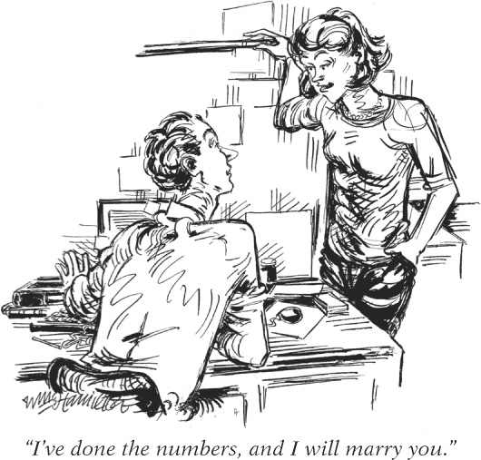
Let’s return to Ashley Hildreth. Assume that Ashley faces the choice of either completing a two-year full-time graduate program in teaching or spending those two years working in her original field of advertising. We’ll also assume that in order to be certified as a teacher, she must complete the entire two years of the graduate program. Which choice should she make?

To get started, let’s consider what Ashley gains by getting the teaching degree—what we might call her revenue from the teaching degree. Once she has completed her degree two years from now, she will receive earnings from her degree valued at $600,000 over the rest of her lifetime. In contrast, if she doesn’t get the degree and stays in advertising, two years from now her future lifetime earnings will be valued at $500,000. The cost of the tuition for her teaching degree program is $40,000, which she pays for with a student loan that costs her $4,000 in interest.

At this point, what she should do might seem obvious: if she chooses the teaching degree, she gets a lifetime increase in the value of her earnings of $600,000 − $500,000 = $100,000, and she pays $40,000 in tuition plus $4,000 in interest. Doesn’t that mean she makes a profit of $100,000 − $40,000 − $4,000 = $56,000 by getting her teaching degree? This $56,000 is Ashley’s accounting profit from obtaining her teaching degree: her revenue minus her explicit cost. In this example her explicit cost of getting the degree is $44,000, the amount of her tuition plus student loan interest.

Although accounting profit is a useful measure, it would be misleading for Ashley to use it alone in making her decision. To make the right decision, the one that leads to the best possible economic outcome for her, she needs to calculate her economic profit—the revenue she receives from the teaching degree minus her opportunity cost of staying in school (which is equal to her explicit cost plus her implicit cost). In general, the economic profit of a given project will be less than the accounting profit because there are almost always implicit costs in addition to explicit costs.

The New Yorker Collection. 2000 William Hamilton from cartoonbank.com. All Rights Reserved

When economists use the term profit, they are referring to economic profit, not accounting profit. This will be our convention in the rest of the book: when we use the term profit, we mean economic profit.

How does Ashley’s economic profit from staying in school differ from her accounting profit? We’ve already encountered one source of the difference: her two years of forgone job earnings. This is an implicit cost of going to school full time for two years. We assume that Ashley’s total forgone earnings for the two years is $57,000.

Once we factor in implicit costs and calculate her economic profit, we see that she is better off not getting a teaching degree. You can see this in Table 18-2: her economic profit from getting the teaching degree is −$1,000. In other words, she incurs an economic loss of $1,000 if she gets the degree. Clearly, she is better off sticking to advertising and going to work now.

To make sure that the concepts of opportunity costs and economic profit are well understood, let’s consider a slightly different scenario. Let’s suppose that Ashley does not have to take out $40,000 in student loans to pay her tuition. Instead, she can pay for it with an inheritance from her grandmother. As a result, she doesn’t have to pay $4,000 in interest. In this case, her accounting profit is $60,000 rather than $56,000. Would the right decision now be for her to get the teaching degree? Wouldn’t the economic profit of the degree now be $60,000 − $57,000 = $3,000?

The answer is no, because Ashley is using her own capital to finance her education, and the use of that capital has an opportunity cost even when she owns it. Capital is the total value of the assets of an individual or a firm. An individual’s capital usually consists of cash in the bank, stocks, bonds, and the ownership value of real estate such as a house. In the case of a business, capital also includes its equipment, its tools, and its inventory of unsold goods and used parts. (Economists like to distinguish between financial assets, such as cash, stocks, and bonds, and physical assets, such as buildings, equipment, tools, and inventory.)

The point is that even if Ashley owns the $40,000, using it to pay tuition incurs an opportunity cost—what she forgoes in the next best use of that $40,000. If she hadn’t used the money to pay her tuition, her next best use of the money would have been to deposit it in a bank to earn interest. To keep things simple, let’s assume that she earns $4,000 on that $40,000 once it is deposited in a bank. Now, rather than pay $4,000 in explicit costs in the form of student loan interest, Ashley incurs $4,000 in implicit costs from the forgone interest she could have earned.

This $4,000 in forgone interest earnings is what economists call the implicit cost of capital—the income the owner of the capital could have earned if the capital had been employed in its next best alternative use. The net effect is that it makes no difference whether Ashley finances her tuition with a student loan or by using her own funds. This comparison reinforces how carefully you must keep track of opportunity costs when making a decision.

Making “Either–Or” Decisions

An “either–or” decision is one in which you must choose between two activities. That’s in contrast to a “how much” decision, which requires you to choose how much of a given activity to undertake. For example, Ashley faced an “either–or” decision: to spend two years in graduate school to obtain a teaching degree, or to work. In contrast, a “how much” decision would be deciding how many hours to study or how many hours to work at a job. Table 18-3 contrasts a variety of “either–or” and “how much” decisions.

In making economic decisions, as we have already emphasized, it is vitally important to calculate opportunity costs correctly. The best way to make an “either–or” decision, the method that leads to the best possible economic outcome, is the straightforward principle of “either–or” decision making. According to this principle, when making an “either–or” choice between two activities, choose the one with the positive economic profit.

Let’s examine Ashley’s dilemma from a different angle to understand how this principle works. If she continues with advertising and goes to work immediately, the total value of her lifetime earnings is $57,000 (her earnings over the next two years) + $500,000 (the value of her lifetime earnings thereafter) = $557,000. If she gets her teaching degree instead and works as a teacher, the total value of her lifetime earnings is $600,000 (value of her lifetime earnings after two years in school) − $40,000 (tuition) − $4,000 (interest payments) = $556,000. The economic profit from continuing in advertising versus becoming a teacher is $557,000 − $556,000 = $1,000.

So the right choice for Ashley is to begin work in advertising immediately, which gives her an economic profit of $1,000, rather than become a teacher, which would give her an economic profit of −$1,000. In other words, by becoming a teacher she loses the $1,000 economic profit she would have gained by working in advertising immediately.

In making “either–or” decisions, mistakes most commonly arise when people or businesses use their own assets in projects rather than rent or borrow assets. That’s because they fail to account for the implicit cost of using self-owned capital. In contrast, when they rent or borrow assets, these rental or borrowing costs show up as explicit costs. If, for example, a restaurant owns its equipment and tools, it would have to compute its implicit cost of capital by calculating how much the equipment could be sold for and how much could be earned by using those funds in the next best alternative project. In addition, businesses run by the owner (an entrepreneur) often fail to calculate the opportunity cost of the owner’s time in running the business. In that way, small businesses often underestimate their opportunity costs and overestimate their economic profit of staying in business.

Making “How Much” Decisions: The Role of Marginal Analysis

Although many decisions in economics are “either–or,” many others are “how much.” Not many people will give up their cars if the price of gasoline goes up, but many people will drive less. How much less? A rise in corn prices won’t necessarily persuade a lot of people to take up farming for the first time, but it will persuade farmers who are already growing corn to plant more. How much more?

To understand “how much” decisions, we will use an approach known as marginal analysis. Marginal analysis involves comparing the benefit of doing a little bit more of some activity with the cost of doing a little bit more of that activity. The benefit of doing a little bit more of something is what economists call its marginal benefit, and the cost of doing a little bit more of something is its marginal cost.

To make his decision, Alex will need to compare the benefit of additional years of schooling with the cost of spending more time in school.

Wavebreakmedia/Shutterstock

Why is this called “marginal” analysis? A margin is an edge; what you do in marginal analysis is push out the edge a bit and see whether that is a good move. We will study marginal analysis by considering a hypothetical decision of how many years of school to complete. We’ll consider the case of Alex, who studies computer programming and design. Since there are many computer languages, app design methods, and graphics programs that can be learned one year at a time, each year Alex can decide whether to continue his studies or not.

Unlike Ashley, who faced an “either–or” decision of whether to get a teaching degree, Alex faces a “how much” decision of how many years to study computer programming and design. For example, he could study one more year, or five more years, or any number of years in between. We’ll begin our analysis of Alex’s decision problem by defining Alex’s marginal cost of another year of study.

Marginal Cost

We’ll assume that each additional year of schooling costs Alex $10,000 in explicit costs—tuition, interest on a student loan, and so on. In addition to the explicit costs, he also has implicit costs—the income forgone by spending one more year in school. Unlike Alex’s explicit costs, which are constant (that is, the same each year), Alex’s implicit cost changes each year. That’s because each year he spends in school leaves him better trained than the year before; and the better trained he is, the higher the salary he can command. Consequently, the income he forgoes by not working rises each additional year he stays in school.

Table 18-4 contains the data on how Alex’s cost of an additional year of schooling changes as he completes more years. The second column shows how his total cost of schooling changes as the number of years he has completed increases. For example, Alex’s first year has a total cost of $30,000: $10,000 in explicit costs of tuition and the like as well as $20,000 in forgone salary.

18-4
Alex’s Marginal Cost of Additional Years in School

The second column also shows that the total cost of attending two years is $70,000: $30,000 for his first year plus $40,000 for his second year. During his second year in school, his explicit costs have stayed the same ($10,000) but his implicit cost of forgone salary has gone up to $30,000. That’s because he’s a more valuable worker with one year of schooling under his belt than with no schooling. Likewise, the total cost of three years of schooling is $130,000: $30,000 in explicit cost for three years of tuition (at $10,000 per year), plus $100,000 in implicit cost of three years of forgone salary. The total cost of attending four years is $220,000, and $350,000 for five years.

The change in Alex’s total cost of schooling when he goes to school an additional year is his marginal cost of the one-year increase in years of schooling. In general, the marginal cost of producing a good or service (in this case, producing one’s own education) is the additional cost incurred by producing one more unit of that good or service. The arrows, which zigzag between the total costs in the second column and the marginal costs in the third column, are there to help you to see how marginal cost is calculated from total cost, and vice versa.

Alex’s marginal costs of more years of schooling have a clear pattern: they are increasing. They go from $30,000, to $40,000, to $60,000, to $90,000, and finally to $130,000 for the fifth year of schooling. That’s because each year of schooling would make Alex a more valuable and highly paid employee if he were to work. As a result, forgoing a job becomes more and more costly as he becomes more educated. This is an example of what economists call increasing marginal cost, which occurs when each unit of a good costs more to produce than the previous unit.

Figure 18-1 shows a marginal cost curve, a graphic representation of Alex’s marginal costs. The height of each shaded bar corresponds to the marginal cost of a given year of schooling. The red line connecting the dots at the midpoint of the top of each bar is Alex’s marginal cost curve. Alex has an upward-sloping marginal cost curve because he has increasing marginal cost of additional years of schooling.

FIGURE18-1Marginal Cost

The height of each shaded bar corresponds to Alex’s marginal cost of an additional year of schooling. The height of each bar is higher than the preceding one because each year of schooling costs more than the previous years. As a result, Alex has increasing marginal cost and the marginal cost curve, the line connecting the midpoints at the top of each bar, is upward sloping.

Although increasing marginal cost is a frequent phenomenon in real life, it’s not the only possibility. Constant marginal cost occurs when the cost of producing an additional unit is the same as the cost of producing the previous unit. Plant nurseries, for example, typically have constant marginal cost—the cost of growing one more plant is the same, regardless of how many plants have already been produced. With constant marginal cost, the marginal cost curve is a horizontal line.

There can also be decreasing marginal cost, which occurs when marginal cost falls as the number of units produced increases. With decreasing marginal cost, the marginal cost line is downward sloping. Decreasing marginal cost is often due to learning effects in production: for complicated tasks, such as assembling a new model of a car, workers are often slow and mistake-prone when assembling the earliest units, making for higher marginal cost on those units. But as workers gain experience, assembly time and the rate of mistakes fall, generating lower marginal cost for later units. As a result, overall production has decreasing marginal cost.

Finally, for the production of some goods and services the shape of the marginal cost curve changes as the number of units produced increases. For example, auto production is likely to have decreasing marginal costs for the first batch of cars produced as workers iron out kinks and mistakes in production. Then production has constant marginal costs for the next batch of cars as workers settle into a predictable pace. But at some point, as workers produce more and more cars, marginal cost begins to increase as they run out of factory floor space and the auto company incurs costly overtime wages. This gives rise to what we call a “swoosh”-shaped marginal cost curve—a topic we will discuss in more detail in the next section. For now, we’ll stick to the simpler example of an increasing marginal cost curve.

Marginal Benefit

Alex benefits from higher lifetime earnings as he completes more years of school. Exactly how much he benefits is shown in Table 18-5. Column 2 shows Alex’s total benefit according to the number of years of school completed, expressed as the value of the increase in lifetime earnings. The third column shows Alex’s marginal benefit from an additional year of schooling. In general, the marginal benefit of producing a good or service is the additional benefit earned from producing one more unit.

18-5
Alex’s Marginal Benefit of Additional Years in School

As in Table 18-4, the data in the third column of Table 18-5 show a clear pattern. However, this time the numbers are decreasing rather than increasing. The first year of schooling gives Alex a $300,000 increase in the value of his lifetime earnings. The second year also gives him a positive return, but the size of that return has fallen to $150,000; the third year’s return is also positive, but its size has fallen yet again to $90,000; and so on. In other words, the more years of school that Alex has already completed, the smaller the increase in the value of his lifetime earnings from attending one more year. Alex’s schooling decision has what economists call decreasing marginal benefit: each additional year of school yields a smaller benefit than the previous year. Or, to put it slightly differently, with decreasing marginal benefit, the benefit from producing one more unit of the good or service falls as the quantity already produced rises.

Just as marginal cost can be represented by a marginal cost curve, marginal benefit can be represented by a marginal benefit curve, shown in blue in Figure 18-2. Alex’s marginal benefit curve slopes downward because he faces decreasing marginal benefit from additional years of schooling. Note, however that not all goods or activities exhibit decreasing marginal benefit.

FIGURE18-2Marginal Benefit

The height of each shaded bar corresponds to Alex’s marginal benefit of an additional year of schooling. The height of each bar is lower than the one preceding it because an additional year of schooling has decreasing marginal benefit. As a result, Alex’s marginal benefit curve, the curve connecting the midpoints at the top of each bar, is downward sloping.

Now we are ready to see how the concepts of marginal benefit and marginal cost are brought together to answer the question of how many years of additional schooling Alex should undertake.

Marginal Analysis

Table 18-6 shows the marginal cost and marginal benefit numbers from Tables 18-4 and 18-5. It also adds an another column: the additional profit to Alex from staying in school one more year, equal to the difference between the marginal benefit and the marginal cost of that additional year in school. (Remember that it is Alex’s economic profit that we care about, not his accounting profit.) We can now use Table 18-6 to determine how many additional years of schooling Alex should undertake in order to maximize his total profit.

18-6
Alex’s Profit from Additional Years of Schooling

First, imagine that Alex chooses not to attend any additional years of school. We can see from column 4 that this is a mistake if Alex wants to achieve the highest total profit from his schooling—the sum of the additional profits generated by another year of schooling. If he attends one additional year of school, he increases the value of his lifetime earnings by $270,000, the profit from the first additional year attended.

Now, let’s consider whether Alex should attend the second year of school. The additional profit from the second year is $110,000, so Alex should attend the second year as well. What about the third year? The additional profit from that year is $30,000; so, yes, Alex should attend the third year as well. What about a fourth year? In this case, the additional profit is negative: it is −$30,000. Clearly, Alex is worse off by attending the fourth additional year rather than taking a job. And the same is true for the fifth year as well: it has a negative additional profit of −$80,000.

What have we learned? That Alex should attend three additional years of school and stop at that point. Although the first, second, and third years of additional schooling increase the value of his lifetime earnings, the fourth and fifth years diminish it. So three years of additional schooling lead to the quantity that generates the maximum possible total profit. It is what economists call the optimal quantity—the quantity that generates the maximum possible total profit.

Figure 18-3 shows how the optimal quantity can be determined graphically. Alex’s marginal benefit and marginal cost curves are shown together. If Alex chooses fewer than three additional years (that is, years 0, 1, or 2), he will choose a level of schooling at which his marginal benefit curve lies above his marginal cost curve. He can make himself better off by staying in school. If instead he chooses more than three additional years (years 4 or 5), he will choose a level of schooling at which his marginal benefit curve lies below his marginal cost curve. He can make himself better off by not attending the additional year of school and taking a job instead.

FIGURE18-3Alex’s Optimal Quantity of Years of Schooling

The optimal quantity is the quantity that generates the highest possible total profit. It is the quantity at which marginal benefit is greater than or equal to marginal cost. Equivalently, it is the quantity at which the marginal benefit and marginal cost curves intersect. Here, they intersect at 3 additional years of schooling. The table confirms that 3 is indeed the optimal quantity: it leads to the maximum total profit of $410,000.

The table in Figure 18-3 confirms our result. The second column repeats information from Table 18-6, showing Alex’s marginal benefit minus marginal cost—the additional profit per additional year of schooling. The third column shows Alex’s total profit for different years of schooling. The total profit, for each possible year of schooling is simply the sum of numbers in the second column up to and including that year. For example, Alex’s profit from additional years of schooling is $270,000 for the first year and $110,000 for the second year. So the total profit for two additional years of schooling is $270,000 + $110,000 = $380,000. Similarly, the total profit for three additional years is $270,000 + $110,000 + $30,000 = $410,000. Our claim that three years is the optimal quantity for Alex is confirmed by the data in the table in Figure 18-3: at three years of additional schooling, Alex reaps the greatest total profit, $410,000.

Alex’s decision problem illustrates how you go about finding the optimal quantity when the choice involves a small number of quantities. (In this example, one through five years.) With small quantities, the rule for choosing the optimal quantity is: increase the quantity as long as the marginal benefit from one more unit is greater than the marginal cost, but stop before the marginal benefit becomes less than the marginal cost.

How many years of schooling will maximize your total profit?

Purestock/Thinkstock

In contrast, when a “how much” decision involves relatively large quantities, the rule for choosing the optimal quantity simplifies to this: The optimal quantity is the quantity at which marginal benefit is equal to marginal cost.

With very large quantities, increasing output by one unit will produce very small changes in marginal benefit and marginal cost. To see why this is so, consider the example of a farmer who finds that her optimal quantity of wheat produced is 5,000 bushels. Typically, she will find that in going from 4,999 to 5,000 bushels, her marginal benefit is only very slightly greater than her marginal cost—that is, the difference between marginal benefit and marginal cost is close to zero. Similarly, in going from 5,000 to 5,001 bushels, her marginal cost is only very slightly greater than her marginal benefit—again, the difference between marginal cost and marginal benefit is very close to zero. So a simple rule in choosing the optimal quantity is to produce the quantity at which the difference between marginal benefit and marginal cost is approximately zero—that is, the quantity at which marginal benefit equals marginal cost.

Now we are ready to state the general rule for choosing the optimal quantity—one that applies for decisions involving either small quantities or large quantities. This general rule is known as the profit-maximizing principle of marginal analysis: When making a profit-maximizing “how much” decision, the optimal quantity is the largest quantity at which marginal benefit is greater than or equal to marginal cost.

The profit-maximizing principle of marginal analysis can be applied to just about any “how much” decision in which you want to maximize the total profit for an activity. It is equally applicable to production decisions, consumption decisions, and policy decisions. Furthermore, decisions where the benefits and costs are not expressed in dollars and cents can also be made using marginal analysis, as long as benefits and costs can be measured in some type of common units. Here are a few examples of decisions that are suitable for marginal analysis:

• A producer, the retailer PalMart, must decide on the size of the new store it is constructing in Beijing. It makes this decision by comparing the marginal benefit of enlarging the store by 1 square foot (the value of the additional sales it makes from that additional square foot of floor space) to the marginal cost (the cost of constructing and maintaining the additional square foot). The optimal store size for PalMart is the largest size at which marginal benefit is greater than or equal to marginal cost.
• Many useful drugs have side effects that depend on the dosage. So a physician must consider the marginal cost, in terms of side effects, of increasing the dosage of a drug versus the marginal benefit of improving health by increasing the dosage. The optimal dosage level is the largest level at which the marginal benefit of disease amelioration is greater than or equal to the marginal cost of side effects.
• A farmer must decide how much fertilizer to apply. More fertilizer increases crop yield but also costs more. The optimal amount of fertilizer is the largest quantity at which the marginal benefit of higher crop yield is greater than or equal to the marginal cost of purchasing and applying more fertilizer.

Sunk Costs

When making decisions, knowing what to ignore can be as important as what to include. Although we have devoted much attention in this module to costs that are important to take into account when making a decision, some costs should be ignored when doing so. Let’s now look at the kinds of costs that people should ignore when making decisions—what economists call sunk costs—and why they should be ignored.

The $250 you already spent on brake pads is irrelevant because it is a sunk cost.

Daniel Grill/Getty Images

To gain some intuition, consider the following scenario. You own a car that is a few years old, and you have just replaced the brake pads at a cost of $250. But then you find out that the entire brake system is defective and also must be replaced. This will cost you an additional $1,500. Alternatively, you could sell the car and buy another of comparable quality, but with no brake defects, by spending an additional $1,600. What should you do: fix your old car, or sell it and buy another?

Some might say that you should take the latter option. After all, this line of reasoning goes, if you repair your car, you will end up having spent $1,750: $1,500 for the brake system and $250 for the brake pads. If instead you sell your old car and buy another, you would spend only $1,600.

But this reasoning, although it sounds plausible, is wrong. It is wrong because it ignores the fact that you have already spent $250 on brake pads, and that $250 cannot be recovered. Therefore, it should be ignored and should have no effect on your decision whether or not to repair your car and keep it. From a rational viewpoint, the real cost at this time of repairing and keeping your car is $1,500, not $1,750. So the correct decision is to repair your car and keep it rather than spend $1,600 on a new car.

In this example, the $250 that has already been spent and cannot be recovered is what economists call a sunk cost. Sunk costs should be ignored in making decisions about future actions because they have no influence on their actual costs and benefits. It’s like the old saying, “There’s no use crying over spilled milk”: once something can’t be recovered, it is irrelevant in making decisions about what to do in the future.

It is often psychologically hard to ignore sunk costs. And if, in fact, you haven’t yet incurred the costs, then you should take them into consideration. That is, if you had known at the beginning that it would cost $1,750 to repair your car, then the right choice at that time would have been to replace the car for $1,600. But once you have already paid the $250 for brake pads, you should no longer include it in your decision making about your next actions. It may be hard to accept that “bygones are bygones,” but it is the right way to make a decision.

18

Check Your Understanding

1. Karma and Don run a furniture-refinishing business from their home. Which of the following represent an explicit cost of the business and which represent an implicit cost?

• a. Supplies such as paint stripper, varnish, polish, sandpaper, and so on

  Supplies are an explicit cost because they require an outlay of money.

• b. Basement space that has been converted into a workroom

  If the basement could be used in some other way that generates money, such as renting it to a student, then the implicit cost is that money forgone. Otherwise, the implicit cost is zero.

• c. Wages paid to a part-time helper

  Wages are an explicit cost.

• d. A van that they inherited and use only for transporting furniture

  By using the van for their business, Karma and Don forgo the money they could have gained by selling it. So use of the van is an implicit cost.

• e. The job at a larger furniture restorer that Karma gave up in order to run the business

  Karma’s forgone wages from her job are an implicit cost.

2. Ashley Hildreth faced the choice of either completing a two-year graduate program in teaching or working at a job in advertising. Assume that she has a third alternative to consider: entering a two-year apprenticeship program for skilled machinists that would, upon completion, make her a licensed machinist. During the apprenticeship, she earns a reduced salary of $15,000 per year. At the end of the apprenticeship, the value of her lifetime earnings is $725,000. What is Ashley’s best career choice?

We need only compare the choice of becoming a machinist to the choice of taking a job in advertising in order to make the right choice. We can discard the choice of acquiring a teaching degree because we already know that taking a job in advertising is always superior to it. Now let’s compare the remaining two alternatives: becoming a skilled machinist versus immediately taking a job in advertising. As an apprentice machinist, Ashley will earn only $30,000 over the first two years, versus $57,000 in advertising. So she has an implicit cost of $30,000 −$57,000 = − $27,000 by becoming a machinist instead of immediately working in advertising. However, two years from now the value of her lifetime earnings as a machinist is $725,000 versus $600,000 in advertising, giving her an accounting profit of $125,000 by choosing to be a machinist. Summing, her economic profit from choosing a career as a machinist over a career in advertising is $125,000 − $27,000 = $98,000. In contrast, her economic profit from choosing the alternative, a career in advertising over a career as a machinist, is −$125,000 + $27,000 = −$98,000. By the principle of “either − or” decision making, Ashley should choose to be a machinist because that career has a positive economic profit.

3. Suppose you have three alternatives—A, B, and C—and you can undertake only one of them. In comparing A versus B, you find that B has an economic profit and A yields an economic loss. But in comparing A versus C, you find that C has an economic profit and A yields an economic loss. How do you decide what to do?

You can discard alternative A because both B and C are superior to it. But you must now compare B versus C. You should then choose the alternative—B or C—that carries a positive economic profit.

4. For each of the “how much” decisions listed in Table 18-3, describe the nature of the marginal cost and of the marginal benefit.

a. The marginal cost of doing your laundry is any monetary outlays plus the opportunity cost of your time spent doing laundry today—that is, the value you would place on spending time today on your next best alternative activity, like seeing a movie. The marginal benefit is having more clean clothes today to choose from.
b. The marginal cost of changing your oil is the opportunity cost of time spent changing your oil now as well as the explicit cost of the oil change. The marginal benefit is the improvement in your car’s performance.
c. The marginal cost is the unpleasant feeling of a burning mouth that you receive from it plus any explicit cost of the jalapeno. The marginal benefit of another jalapeno on your nachos is the pleasant taste that you receive from it.
d. The marginal benefit of hiring another worker in your company is the value of the output that worker produces. The marginal cost is the wage you must pay that worker.
e. The marginal cost is the value lost due to the increased side effects from this additional dose. The marginal benefit of another dose of the drug is the value of the reduction in the patient’s disease.
f. The marginal cost is the opportunity cost of your time— what you would have gotten from the next best use of your time. The marginal benefit is the probable increase in your grade.

5. Suppose that Alex’s school charges a fixed fee of $70,000 for four years of schooling. If Alex drops out before he finishes those four years, he still has to pay the $70,000. Alex’s total cost for different years of schooling is now given by the data in the accompanying table. Assume that Alex’s total benefit and marginal benefit remain as reported in Table 18-5.
Use this information to calculate (i) Alex’s new marginal cost, (ii) his new profit, and (iii) his new optimal years of schooling. What kind of marginal cost does Alex now have—constant, increasing, or decreasing?

Quantity of schooling (years)	Total cost
0	$0
1	90,000
2	120,000
3	170,000
4	250,000
5	370,000

The accompanying table shows Alex’s new marginal cost and his new profit. It also reproduces Alex’s marginal benefit from Table 18-5.

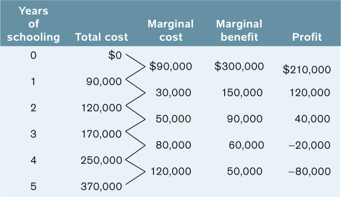
Alex’s marginal cost is decreasing until he has completed two years of schooling, after which marginal cost increases because of the value of his forgone income. The optimal amount of schooling is still three years. For less than three years of schooling, marginal benefit exceeds marginal cost; for more than three years, marginal cost exceeds marginal benefit.

6. You have decided to go into the ice-cream business and have bought a used ice-cream truck for $8,000. Now you are reconsidering. What is your sunk cost in the following scenarios?

• a. The truck cannot be resold.

  Your sunk cost is $8,000 because none of the $8,000 spent on the truck is recoverable.

• b. The truck can be resold, but only at a 50% discount.

  Your sunk cost is $4,000 because 50% of the $8,000 spent on the truck is recoverable.

7. You have gone through two years of medical school but are suddenly wondering whether you wouldn’t be happier as a musician. Which of the following statements are potentially valid arguments and which are not?

• a. “I can’t give up now, after all the time and money I’ve put in.”

  This is an invalid argument because the time and money already spent are a sunk cost at this point.

• b. “If I had thought about it from the beginning, I never would have gone to med school, so I should give it up now.”

  This is also an invalid argument because what you should have done two years ago is irrelevant to what you should do now.

• c. “I wasted two years, but never mind—let’s start from here.”

  This is a valid argument because it recognizes that sunk costs are irrelevant to what you should do now.

• d. “My parents would kill me if I stopped now.” (Hint: We’re discussing your decision-making ability, not your parents’.)

  This is a valid argument given that you are concerned about disappointing your parents. But your parents’ views are irrational because they do not recognize that the time already spent is a sunk cost.

You and your friend are at the stadium watching your favorite football team. But they are losing so badly that you can’t bear to watch anymore and want to leave. Your friend, however, says, “But we paid $100 for these seats. Shouldn’t we stay and get our money’s worth?” How do you respond?

MUDDLED AT THE MARGIN

The idea of setting marginal benefit equal to marginal cost sometimes confuses people. Aren’t we trying to maximize the difference between benefits and costs? And don’t we wipe out our gains by setting benefits and costs equal to each other?

The answer to both questions is yes. But this is not what we are doing. Rather, what we are doing is setting marginal, not total, benefit and cost equal to each other. Once again, the point is to maximize the total profit from an activity. If the marginal benefit from the activity is greater than the marginal cost, doing a bit more will increase that profit. If the marginal benefit is less than the marginal cost, doing a bit less will increase the total profit. So only when the marginal benefit and marginal cost are equal is the difference between total benefit and total cost at a maximum.

To learn more about the idea of setting marginal benefit equal to marginal cost, see pages 198–200 on marginal analysis, and Figure 18-3.