14.2 Solving the Dynamic Model
We have now looked at each of the pieces of the dynamic AD–AS model. To summarize, here are the five equations that make up the model:
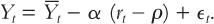
Yt =  – α (rt – ρ) +ϵt
 |
The Demand for Goods and Services |
| rt = it – Etπt+1 | The Fisher Equation |
| πt = Et+1πt+ ϕ(Yt –
) + vt |
The Phillips Curve |
| Etπt+1 = πt | Adaptive Expectations |
| it = πt + ρ + θπ(πt – π*t) + θY(Yt –
) |
The Monetary-Policy Rule |
These five equations determine the paths of the model’s five endogenous variables: output Yt, the real interest rate rt, inflation πt, expected inflation Etπt+1, and the nominal interest rate it.
Table 14-1 lists all the variables and parameters in the model. In any period, the five endogenous variables are influenced by the four exogenous variables in the equations as well as the previous period’s inflation rate. Lagged inflation πt–1 is called a predetermined variable. That is, it is a variable that was endogenous in the past but, because it is fixed by the time when we arrive in period t, is essentially exogenous for the purposes of finding the current equilibrium.
| Endogenous Variables | |
| Yt | Output |
| πt | Inflation |
| rt | Real interest rate |
| it | Nominal interest rate |
| Etπt+1 | Expected inflation |
| Exogenous Variables | |
|
|
Natural level of output |
| πt* | Central bank’s target for inflation |
| ϵt | Shock to the demand for goods and services |
| vt | Shock to the Phillips curve (supply shock) |
| Predetermined Variable | |
| πt–1 | Previous period’s inflation |
| Parameters | |
| α | The responsiveness of the demand for goods and services to the real interest rate |
| ρ | The natural rate of interest |
| ϕ | The responsiveness of inflation to output in the Phillips curve |
| θπ | The responsiveness of the nominal interest rate to inflation in the monetary-policy rule |
| θY | The responsiveness of the nominal interest rate to output in the monetary-policy rule |
We are almost ready to put these pieces together to see how various shocks to the economy influence the paths of these variables over time. Before doing so, however, we need to establish the starting point for our analysis: the economy’s long-run equilibrium.
The Long-Run Equilibrium
The long-run equilibrium represents the normal state around which the economy fluctuates. It occurs when there are no shocks (ϵt = vt = 0) and inflation has stabilized (πt = πt–1).
Straightforward algebra applied to the above five equations can be used to verify these long-run values:

rt = ρ.
πt = πt*.
Etπt+1 = πt*.
it = ρ + πt*.
In words, the long-run equilibrium is described as follows: output and the real interest rate are at their natural values, inflation and expected inflation are at the target rate of inflation, and the nominal interest rate equals the natural rate of interest plus target inflation.
The long-run equilibrium of this model reflects two related principles: the classical dichotomy and monetary neutrality. Recall that the classical dichotomy is the separation of real from nominal variables, and monetary neutrality is the property according to which monetary policy does not influence real variables. The equations immediately above show that the central bank’s inflation target πt* influences only inflation πt, expected inflation Etπt+1, and the nominal interest rate it. If the central bank raises its inflation target, then inflation, expected inflation, and the nominal interest rate all increase by the same amount. The real variables—output Yt and the real interest rate rt—do not depend on monetary policy. In these ways, the long-run equilibrium of the dynamic AD–AS model mirrors the classical models we examined in Chapters 3 to 8.
The Dynamic Aggregate Supply Curve
To study the behaviour of this economy in the short run, it is useful to analyze the model graphically. Because graphs have two axes, we need to focus on two variables. We will use output Yt and inflation πt as the variables on the two axes because these are the variables of central interest. As in the conventional AD–AS model, output will be on the horizontal axis. But because the price level has faded into the background in this dynamic presentation, the vertical axis in our graphs will now represent the inflation rate.
To generate this graph, we need two equations that summarize the relationships between output Yt and inflation πt. These equations are derived from the five equations of the model we have already seen. To isolate the relationships between Yt and πt, however, we need to use a bit of algebra to eliminate the other three endogenous variables (rt, it, and Et–1πt).
The first relationship between output and inflation comes almost directly from the Phillips curve equation. We can get rid of the one extra endogenous variable in the equation (Et–1πt) by using the expectations equation (Et–1πt = πt–1) to substitute past inflation πt–1 for expected inflation Et–1πt. With this substitution, the equation for the Phillips curve becomes

This equation relates inflation πt and output Yt for given values of two exogenous variables (
and vt) and a predetermined variable (πt–1).
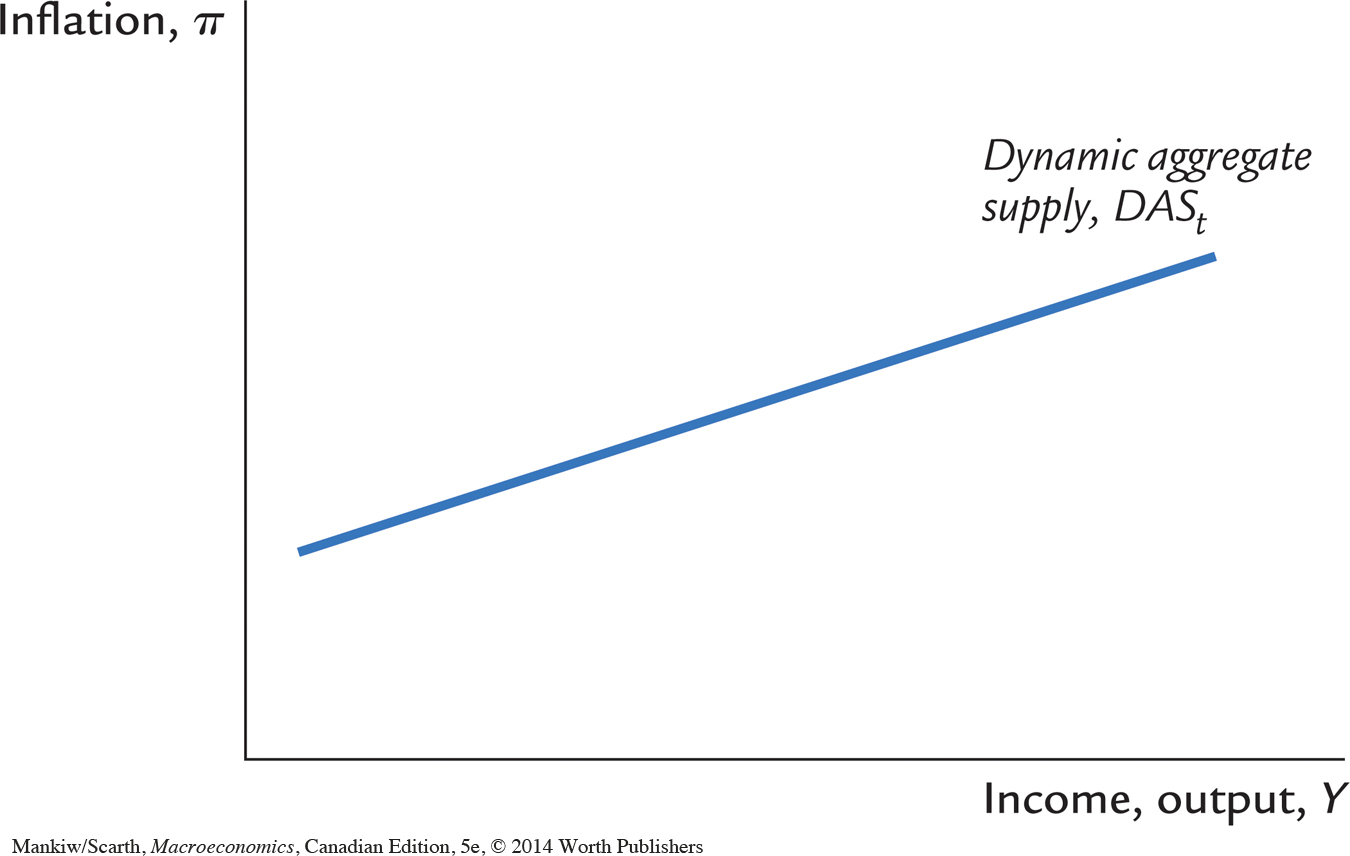
Figure 14-2 graphs the relationship between inflation πt and output Yt described by this equation. We call this upward-sloping curve the dynamic aggregate supply curve, or DAS. The dynamic aggregate supply curve is similar to the aggregate supply curve we saw in Chapter 13, except that inflation rather than the price level is on the vertical axis. The DAS curve shows how inflation is related to output in the short run. Its upward slope reflects the Phillips curve: Other things equal, high levels of economic activity are associated with high inflation.
 , and the supply shock vt. When these variables change, the curve shifts.
The DAS curve is drawn for given values of past inflation πt–1, the natural level of output
, and the supply shock vt. If any one of these three variables changes, the DAS curve shifts. One of our tasks ahead is to trace out the implications of such shifts. But first, we need another curve.
The Dynamic Aggregate Demand Curve
The dynamic aggregate supply curve is one of the two relationships between output and inflation that determine the economy’s short-run equilibrium. The other relationship is (no surprise) the dynamic aggregate demand curve. We derive it by combining four equations from the model and then eliminating all the endogenous variables other than output and inflation.
We begin with the demand for goods and services:
To eliminate the endogenous variable rt, the real interest rate, we use the Fisher equation to substitute it – Etπt+1 for rt:

To eliminate another endogenous variable, the nominal interest rate it, we use the monetary-policy equation to substitute for it:

Next, to eliminate the endogenous variable expected inflation Etπt+1, we use our equation for inflation expectations to substitute πt for Etπt+1:

Notice that the positive πt and ρ inside the brackets cancel the negative ones. The equation simplifies to

If we now bring like terms together and solve for Yt, we obtain

This equation relates output Yt to inflation πt for given values of three exogenous variables (
, π*t, and ϵt).
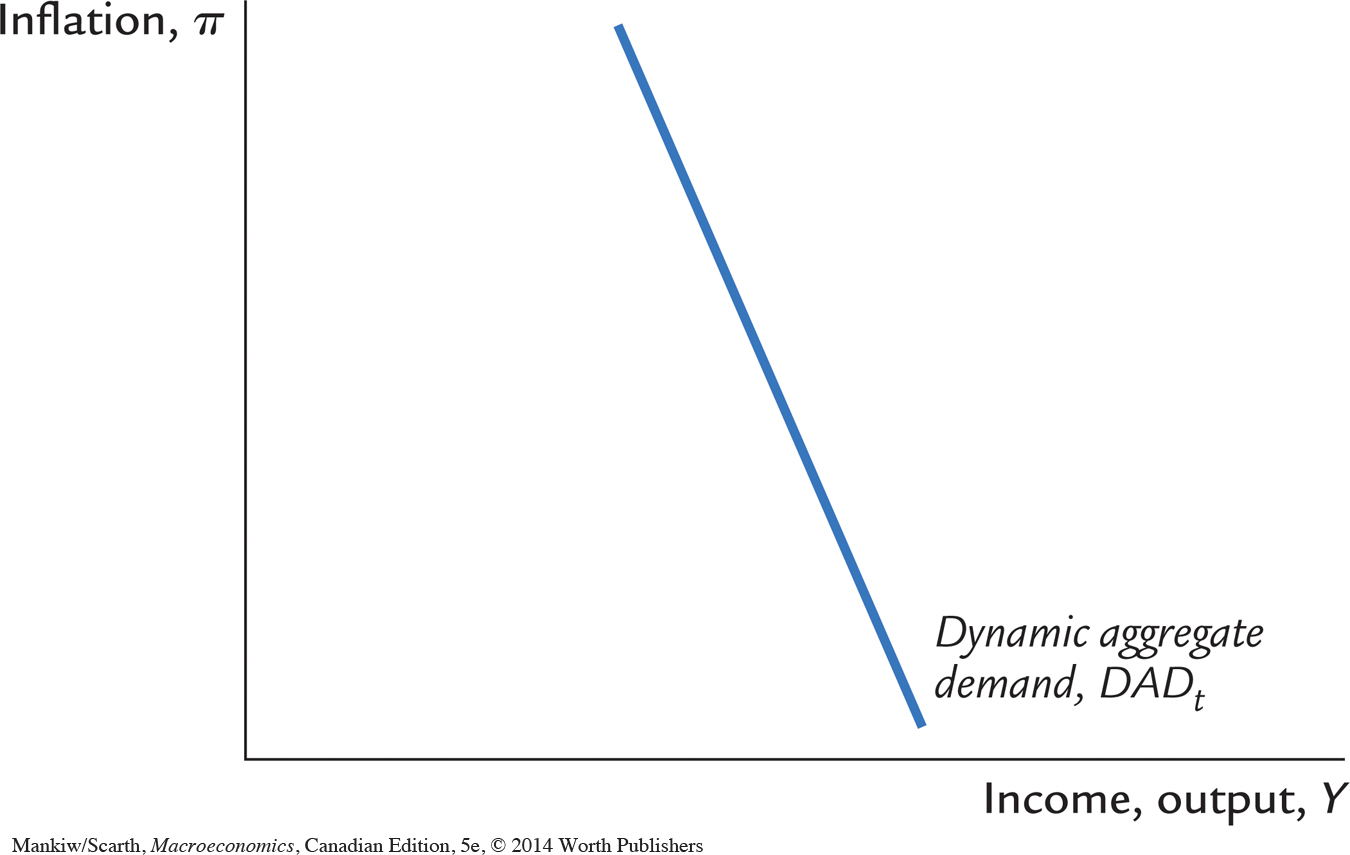
Figure 14-3 graphs the relationship between inflation πt and output Yt described by this equation. We call this downward-sloping curve the dynamic aggregate demand curve, or DAD. The DAD curve shows how the quantity of output demanded is related to inflation in the short run. It is drawn holding constant the natural level of output
, the inflation target πt*, and the demand shock ϵt. If any one of these three variables changes, the DAD curve shifts. We will examine the effect of such shifts shortly.
 , the inflation target πt*, and the demand shock ϵt. When these exogenous variables change, the curve shifts.
It is tempting to think of this dynamic aggregate demand curve as nothing more than the standard aggregate demand curve from Chapter 11 with inflation, rather than the price level, on the vertical axis. In some ways, they are similar: they both embody the link between the interest rate and the demand for goods and services. But there is an important difference. The conventional aggregate demand curve in Chapter 11 is drawn for a given money supply. By contrast, because the monetary-policy rule was used to derive the dynamic aggregate demand equation, the dynamic aggregate demand curve is drawn for a given rule for monetary policy. Under that rule, the central bank sets the interest rate based on macro-economic conditions, and it allows the money supply to adjust accordingly.
The dynamic aggregate demand curve is downward sloping because of the following mechanism. When inflation rises, the central bank follows its rule and responds by increasing the nominal interest rate. Because the rule specifies that the central bank raise the nominal interest rate by more than the increase in inflation, the real interest rate rises as well. The increase in the real interest rate reduces the quantity of goods and services demanded. This negative association between inflation and quantity demanded, working through central bank policy, makes the dynamic aggregate demand curve slope downward.
The dynamic aggregate demand curve shifts in response to changes in fiscal and monetary policy. As we noted earlier, the shock variable ϵt reflects changes in government spending and taxes (among other things). Any change in fiscal policy that increases the demand for goods and services means a positive value of ϵt and a shift of the DAD curve to the right. Any change in fiscal policy that decreases the demand for goods and services means a negative value of ϵt and a shift of the DAD curve to the left.
Monetary policy enters the dynamic aggregate demand curve through the target inflation rate πt*. The DAD equation shows that, other things equal, an increase in πt* raises the quantity of output demanded. (There are two negative signs in front of πt* so the effect is positive.) Here is the mechanism that lies behind this mathematical result: When the central bank raises its target for inflation, it pursues a more expansionary monetary policy by reducing the nominal interest rate. The lower nominal interest rate in turn means a lower real interest rate, which stimulates spending on goods and services. Thus, output is higher for any given inflation rate, so the dynamic aggregate demand curve shifts to the right. Conversely, when the central bank reduces its target for inflation, it raises nominal and real interest rates, thereby dampening demand for goods and services and shifting the dynamic aggregate demand curve to the left.
The Short-Run Equilibrium
The economy’s short-run equilibrium is determined by the intersection of the dynamic aggregate demand curve and the dynamic aggregate supply curve. The economy can be represented algebraically using the two equations we have just derived:
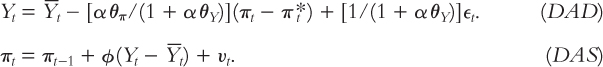
In any period t, these equations together determine two endogenous variables: inflation πt and output Yt. The solution depends on five other variables that are exogenous (or at least determined prior to period t). These exogenous (and predetermined) variables are the natural level of output
, the central bank’s target inflation rate πt*, the shock to demand ϵt, the shock to supply vt, and the previous period’s rate of inflation πt–1.
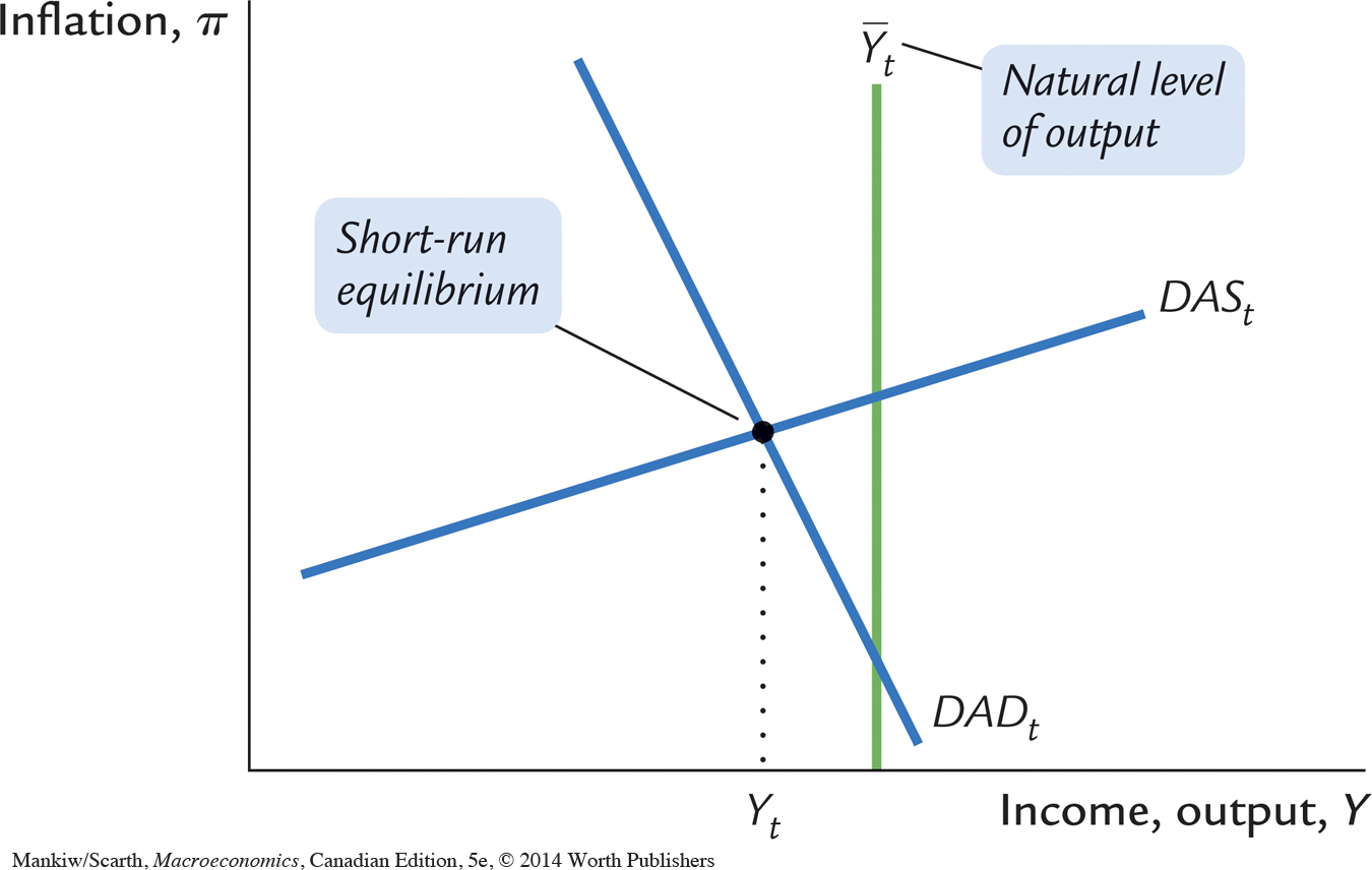
Taking these exogenous variables as given, we can illustrate the economy’s short-run equilibrium as the intersection of the dynamic aggregate demand curve and the dynamic aggregate supply curve, as in Figure 14-4. The short-run equilibrium level of output Yt can be less than its natural level
, as it is in this figure, greater than its natural level, or equal to it. As we have seen, when the economy is in long-run equilibrium, output is at its natural level (Yt =
).
 .
.
The short-run equilibrium determines not only the level of output Yt but also the inflation rate πt. In the subsequent period (t + 1), this inflation rate will become the lagged inflation rate that influences the position of the dynamic aggregate supply curve. This connection between periods generates the dynamic patterns that we will examine below. That is, one period of time is linked to the next through expectations about inflation. A shock in period t affects inflation in period t, which in turn affects the inflation that people expect for period t + 1. Expected inflation in period t + 1 in turn affects the position of the dynamic aggregate supply curve in that period, which in turn affects output and inflation in period t + 1, which then affects expected inflation in period t + 2, and so on.
These linkages of economic outcomes across time periods will become clear as we work through a series of examples.