nolanessentials3e

15.3 Ordinal Data and Correlation

448

The statistical tests we discuss in this section allow researchers to draw conclusions from data that do not meet the assumptions for a parametric test, such as when the data are rank ordered. In this section, we learn how to convert scale data to ordinal data. Then we examine two tests that can be used with ordinal data: the Spearman rank-order correlation coefficient (a nonparametric version of the Pearson correlation coefficient) and the Mann–Whitney U test (a nonparametric version of the independent-samples t test).

When the Data Are Ordinal

A University of Chicago News Office press release proclaimed, “Americans and Venezuelans Lead the World in National Pride.” Researchers from the University of Chicago’s National Opinion Research Center (NORC) surveyed citizens of 33 countries (Smith & Kim, 2006) and developed two different kinds of national pride scores: pride in specific accomplishments of their nations, like science or sports (which they called domain-specific national pride) and a more general national pride in which citizens responded to items such as, “People should support their country even if the country is in the wrong.”

National Pride University of Chicago researchers ranked 33 countries in terms of national pride. Venezuela, along with the United States, came out on top. Ordinal data such as these are analyzed using nonparametric statistics.

AP Photo/Leslie Mazoch

So, the researchers had two sets of national pride scores—accomplishment-related and general—for each country. They converted the scores to ranks, and when results on the two scales were merged, Venezuela and the United States were tied for first place. These findings suggest many hypotheses about what creates and inflates national pride. The authors noted that countries that were settled as colonies tend to rank higher than their “mother country,” that formerly socialist countries tend to rank lower than other countries, and that countries in Asia tend to rank lower than those from other continents. The researchers also reported that there were increases in national pride among countries that had recently been subject to terrorist attacks.

449

We wondered about other possible precursors of national pride, such as competitiveness. Because the researchers provided ordinal data, the only way we can explore these interesting hypotheses is by using nonparametric statistics. Parametric statistics are appropriate for scale data, but they are not appropriate for ordinal data. As we noted earlier in the chapter, the very nature of an ordinal variable means that it will not meet the assumptions of a scale dependent variable and a normally distributed population. As we can see in Figure 15-7, the shape of a distribution of ordinal variables is rectangular because every participant has a different rank.

Figure 15.17: FIGURE 15-7
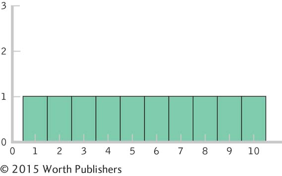
A Histogram of Ordinal Data
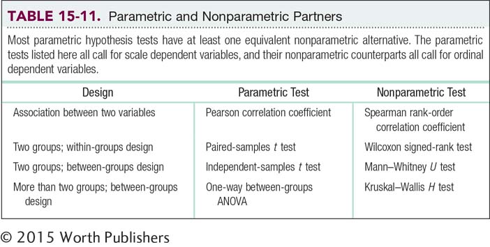
When ordinal data are graphed in a histogram, the resulting distribution is rectangular. These are data for ranks 1–10. For each rank, there is one individual. Ordinal data are never normally distributed.

Fortunately, the logic of many nonparametric statistics will be familiar to students. This is because many of the nonparametric statistical tests are specific alternatives to parametric statistical tests. These nonparametric tests may be used whenever assumptions for a parametric test are not met. For example, four such tests that are commonly used are (shown in Table 15-11): (1) a nonparametric equivalent for the Pearson correlation coefficient, the Spearman rank-order correlation coefficient; (2) a nonparametric equivalent for the paired-samples t test, the Wilcoxon signed-rank test; (3) a nonparametric equivalent for the independent-samples t test, the Mann–Whitney U test; and (4) a nonparametric equivalent for the one-way between-groups ANOVA, the Kruskal–Wallis H test. There is almost always an established nonparametric alterative to a parametric test. When researchers can’t meet the assumptions of the parametric test they would like to conduct, they can choose the nonparametric test that is appropriate for their data. In this chapter, we’ll explore the Spearman rank-order correlation coefficient and the Mann–Whitney U test.

EXAMPLE 15.6

450

Nonparametric tests for ordinal data are typically used in one of two situations. First and most obviously, we use nonparametric tests when the sample data are ordinal. Second, we use nonparametric tests when the dependent variable suggests that the underlying population distribution is greatly skewed, a common situation when the sample size is small. This second reason is likely why the national pride researchers converted their data to ranks (Smith & Kim, 2006). 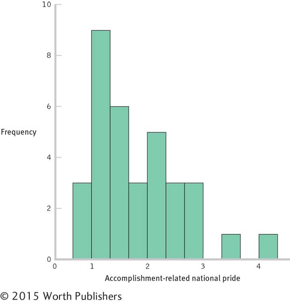Figure 15-8 shows a histogram of their full set of data for the variable accomplishment-related national pride—the variable that we will use for many examples in this chapter. The data appear to be positively skewed, most likely because two countries, Venezuela and the United States, appear to be outliers. Because of this, we have to transform the data from scale to ordinal.

Figure 15.19: FIGURE 15-8
Skewed Data
The sample data for the variable, accomplishment-related national pride, are skewed. This indicates the possibility that the underlying population distribution is skewed. It is likely that the researchers chose to report their data as ranks for this reason (Smith & Kim, 2006).

It is appropriate to transform scale data to ordinal data whenever the data from a small sample are skewed. For example, look what happens to the following five data points for income when we change the data from scale to ordinal. In the first row, the one that includes the scale data, there is a severe outlier ($550,000) and the sample data suggest a skewed distribution. In the second row, the severe outlier merely becomes the last ranking. The ranked data do not have an outlier.

Scale: $24,000 $27,000 $35,000 $46,000 $550,000

Ordinal: 1 2 3 4 5

In the next section, we’ll transform scale data to ordinal data so that we can calculate the Spearman rank-order correlation coefficient.

The Spearman Rank-Order Correlation Coefficient

451

The Spearman rank-order correlation coefficient is a nonparametric statistic that quantifies the association between two ordinal variables.

MASTERING THE CONCEPT

15-4: We calculate a Spearman rank-order correlation coefficient to quantify the association between two ordinal variables. It is the nonparametric equivalent of the Pearson correlation coefficient

Many everyday, automatic decisions are based on rank-ordered observations. For example, a person may prefer Chunky Monkey ice cream to Chubby Hubby ice cream but would not be able to specify that he liked it precisely twice as much. When we collect ranked data, we analyze it using nonparametric statistics. The Spearman rank-order correlation coefficient is a nonparametric statistic that quantifies the association between two ordinal variables.

EXAMPLE 15.7

To see how the Spearman rank-order correlation coefficient works, let’s look at a study that uses two ordinal variables, one taken from the University of Chicago study on national pride (Smith & Kim, 2006). We wondered whether accomplishment-related national pride is related to the underlying trait of competitiveness. So, we randomly selected 10 countries from the university’s list and compiled those countries’ scores for accomplishment-related national pride. We also included rankings of competitiveness that had been compiled by an international business school (IMD International, 2001).

A correlation between these variables, if found, would be evidence that countries’ levels of accomplishment-related national pride are tied to levels of competitiveness. The competitiveness variable we borrowed from the business school rankings was already ordinal. However, the accomplishment-related national pride variable was initially a scale variable. When even one of the variables is ordinal, we use the Spearman rank-order correlation coefficient (often called just the Spearman correlation coefficient, or Spearman’s rho). Its symbol is almost like the one for the Pearson correlation coefficient, but it has a subscript S to indicate that it is Spearman’s correlation coefficient: r_S.

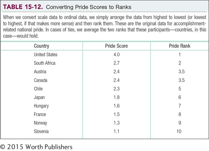
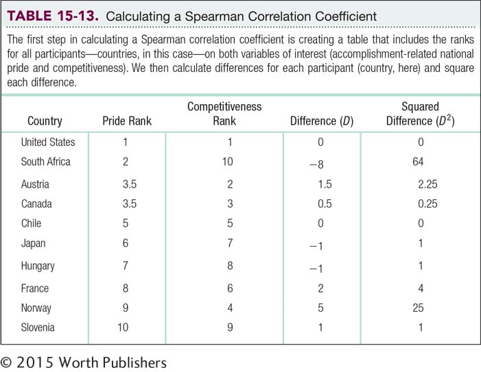
To convert scale data to ordinal data, we simply organize the data from highest to lowest (or lowest to highest, if that makes more sense) and then rank them. Table 15-12 shows the conversion of accomplishment-related national pride from scale data to ordinal data. Sometimes, as seen for Austria and Canada, we have a tie. Both of these countries had an accomplishment-related national pride score of 2.40. When we rank the data, these countries take the third and fourth positions, but they must have the same rank because their scores are the same. So we take the average of the two ranks they would hold if the scores were different: (3 + 4)/2 = 3.5. Both of these countries receive the rank of 3.5.

452

Now that we have the ranks, we can compute the Spearman correlation coefficient. We first need to include both sets of ranks in the same table, as in the second and third columns in Table 15-13. We then calculate the difference (D) between each pair of ranks, as in the fourth column. The differences always add up to 0, so we must square the differences, as in the last column. As we have frequently done with squared differences in the past, we sum them—another variation on the concept of a sum of squares. The sum of these squared differences is:

ΣD² = (0 + 64 + 2.25 + 0.25 + 0 + 1 + 1 + 4 + 25 + 1) = 98.5

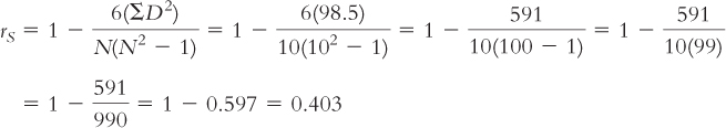
The formula for calculating the Spearman correlation coefficient includes the sum of the squared differences that we just calculated, 98.5. The formula is:

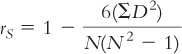
Aside from the sum of squared differences, the only other information we need is the sample size, N, which is 10 in this example. (The number 6 is a constant; it is always included in the calculation of the Spearman correlation coefficient.) The Spearman correlation coefficient, therefore, is:

453

The Spearman correlation coefficient is 0.40.

MASTERING THE FORMULA

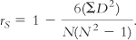
15-6: The formula for the Spearman correlation coefficient is:

The numerator includes a constant, 6, as well as the sum of the squared differences between ranks for each participant. The denominator is calculated by multiplying the sample size, N, by the square of the sample size minus 1.

The interpretation of the Spearman correlation coefficient is identical to that for the Pearson correlation coefficient. The coefficient can range from −1, a perfect negative correlation, to 1, a perfect positive correlation. A correlation coefficient of 0 indicates no relation between the two variables. As with the Pearson correlation coefficient, it is not the sign of the Spearman correlation coefficient that indicates the strength of a relation. So, for example, a coefficient of −0.66 indicates a stronger association than does a coefficient of 0.23. Finally, as with the Pearson correlation coefficient, we can implement the six steps of hypothesis testing to determine whether the Spearman correlation coefficient is statistically significantly different from 0. If we do decide to conduct hypothesis testing, we can find the critical values for the Spearman correlation coefficient in Appendix B.7.

Like the Pearson correlation coefficient, the Spearman correlation coefficient does not tell us about causation. It is possible that there is a causal relation in one of two directions. The relation between competitiveness (variable A) and accomplishment-related national pride (variable B) is 0.40, a fairly strong positive correlation. It is possible that competitiveness (variable A) causes a country to feel prouder (variable B) of its accomplishments. On the other hand, it is also possible that accomplishment-related national pride (variable B) causes competitiveness (variable A). Finally, it is also possible that a third variable, C, causes both of the other two variables (A and B). For example, a high gross domestic product (variable C) might cause both a sense of competitiveness with other economic powerhouses (variable A) and a feeling of national pride at this economic accomplishment (variable B). A strong correlation indicates only a strong association; we can draw no conclusions about causation.

The Mann–Whitney U Test

MASTERING THE CONCEPT

15-5: We conduct a Mann–Whitney U test to compare two independent groups with respect to an ordinal dependent variable. It is the nonparametric equivalent of the independent-samples t test.

The Mann–Whitney U test is a nonparametric hypothesis test used when there are two groups, a between-groups design, and an ordinal dependent variable.

As mentioned earlier, most parametric hypothesis tests have nonparametric equivalents. In this section, we learn how to conduct one of the most common of these tests—the Mann–Whitney U test, the nonparametric equivalent of the independent-samples t test. The Mann-Whitney U test is a nonparametric hypothesis test used when there are two groups, a between-groups design, and an ordinal dependent variable. The test statistic is symbolized as U. Let’s use this new statistic to test more hypotheses about the ranked data on national pride.

EXAMPLE 15.8

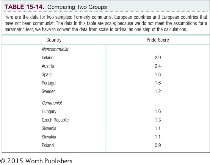
The researchers observed that countries with a recent communist past tended to have lower ranks on national pride (Smith & Kim, 2006). Let’s choose 10 European countries, 5 of which were communist during part of the twentieth century. The independent variable is type of country, with two levels: formerly communist and not formerly communist. The dependent variable is rank on accomplishment-related national pride. As in previous situations, we may start with ordinal data, or we may convert scale data to ordinal data because we were far from meeting the assumptions of a parametric test. Table 15-14 shows the scores for the 10 countries.

454

As noted earlier, nonparametric tests use the same six steps of hypothesis testing as parametric tests but are usually easier to calculate.

STEP 1: Identify the assumptions.

There are three assumptions. (1) The data must be ordinal. (2) We should use random selection; otherwise, the ability to generalize will be limited. (3) Ideally, no ranks are tied. The Mann–Whitney U test is robust with respect to violations of the third assumption; if there are only a few ties, then it is usually safe to proceed.

Summary: (1) We need to convert the data from scale to ordinal. (2) The researchers did not indicate whether they used random selection to choose the European countries in the sample, so we must be cautious when generalizing from these results. (3) There are some ties, but we will assume that there are not so many as to render the results of the test invalid.

STEP 2: State the null and research hypotheses.

We state the null and research hypotheses only in words, not in symbols.

Summary: Null hypothesis: Formerly communist European countries and European countries that have not been communist do not tend to differ in accomplishment-related national pride. Research hypothesis: Formerly communist European countries and European countries that have not been communist tend to differ in accomplishment-related national pride.

STEP 3: Determine the characteristics of the comparison distribution.

The Mann–Whitney U test compares the two distributions—those represented by the two samples. There is no comparison distribution in the sense of a parametric test. To complete step 4 and find a cutoff, or critical value, we need two pieces of information: the sample size for the first group and the sample size for the second group.

455

Summary: There are five countries in the formerly communist group and five countries in the noncommunist group.

STEP 4: Determine the critical values, or cutoffs.

There are two Mann–Whitney U tables. We use Table B.8A (for a one-tailed test) or Table B.8B (for a two-tailed test) from Appendix B to determine the cutoff, or critical value, for the Mann–Whitney U test. In the tables, we find the sample size for the first group across the top row and the sample size for the second group down the left-hand column. The table includes only critical values for a hypothesis test with a p level of 0.05. There are two differences between this critical value and those we considered with parametric tests. First, we calculate two test statistics, but we only compare the smaller one with the critical value. Second, we want the test statistic to be equal to or smaller than the critical value.

Summary: The cutoff, or critical value, for a Mann–Whitney U test with two groups of five participants (countries), a p level of 0.05, and a two-tailed test is 2. (Note: Remember that we want the smaller of the test statistics to be equal to or smaller than this critical value.)

STEP 5: Calculate the test statistic.

As noted above, we calculate two test statistics for a Mann–Whitney U test, one for each group. We start the calculations by organizing the data by raw score from highest to lowest in one single column and then by rank in the next column, as shown in Table 15-15. For the two sets of tied scores, we take the average of the ranks they would have held and apply that rank to the tied scores. For example, Spain, Portugal, and Hungary all received scores of 1.6; they would have been ranked 3, 4, and 5, but because they are tied, they all received the average of these three scores, 4. (We have chosen to give the highest score a rank of 1, as did the researchers.) We include the group membership of each participant (country) next to its score and rank: C indicates a formerly communist country and NC represents a noncommunist country. The final two columns separate the ranks by group; from these columns we can easily see that the noncommunist countries tend to hold the higher ranks and the communist countries, the lower ranks.

456

MASTERING THE FORMULA

15-7: The formula for the first group in a Mann–Whitney U test is:

The formula for the second group is:

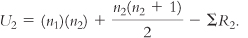
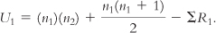
The symbol n refers to the sample size for a particular group. In these formulas, the first group is labeled 1 and the second group is labeled 2. ΣR refers to the sum of the ranks for a particular group.

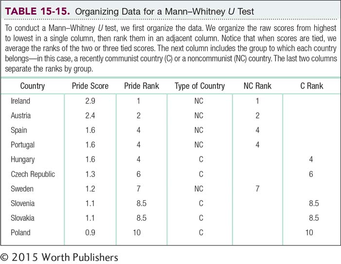
Before we continue, we sum the ranks (R) for each group and add subscripts to indicate which group is which:

ΣR_NC = 1 + 2 + 4 + 4 + 7 = 18

ΣR_C = 4 + 6 + 8.5 + 8.5 + 10 = 37

The formula for the first group, with the n’s referring to sample size in a particular group, is:

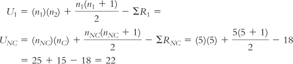
The formula for the second group is:

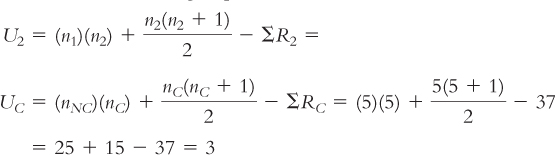
Summary: U_NC = 22; U_C = 3

STEP 6: Make a decision.

For a Mann–Whitney U test, we compare only the smaller test statistic, 3, with the critical value, 2. This test statistic is not smaller than the critical value, so we fail to reject the null hypothesis. We cannot conclude that the two groups are different with respect to accomplishment-related national pride rankings. The researchers concluded, however, that noncommunist countries tend to have more national pride, but remember, the researchers used more countries in their analyses than we did here, so they had more statistical power (Smith & Kim, 2006). We selected just 10 of the European countries on their list. As with parametric tests, increased sample sizes lead to increased statistical power.

Summary: The test statistic, 3, is not smaller than the critical value, 2. We cannot reject the null hypothesis. We conclude only that there is insufficient evidence to show that the two groups are different with respect to accomplishment-related national pride.

After completing the hypothesis test, we want to present the primary statistical information in a report. In the write-up, we list the two groups and their sample sizes, but there are no degrees of freedom. In addition, we report the smaller test statistic; because this is the standard, we do not include a subscript. The statistics read:

U = 3, p > 0.05

(Note: If we conduct the Mann–Whitney U test using software, we report the actual p value associated with the test statistic.)

457

CHECK YOUR LEARNING

Reviewing the Concepts		Nonparametric tests for ordinal data are used when the data are already ordinal or when it is clear that the assumptions are severely violated. In the latter case, the scale data must be converted to ordinal data. When we want to calculate a correlation between two ordinal variables, we calculate a Spearman rank-order correlation coefficient, which is interpreted in the same way as a Pearson correlation coefficient. As with the Pearson correlation coefficient, the Spearman correlation coefficient does not tell us about causation. It simply quantifies the magnitude and direction of association between two ordinal variables. There are nonparametric hypothesis tests that can be used to replace the various parametric hypothesis tests when it seems clear that there are severe violations of the assumptions. We use the Mann–Whitney U test in place of the independent-samples t test. Nonparametric hypothesis tests use the same six steps of hypothesis testing that are used for parametric tests, but the steps and the calculations tend to be simpler.
Clarifying the Concepts	15-11	Describe a common situation in which we use nonparametric tests other than chi-square tests.
	15-12	Why must scale data be transformed into ordinal data before any nonparametric tests are performed?
Calculating the Statistics	15-13	Convert the following scale data to ordinal or ranked data, starting with a rank of 1 for the smallest data point.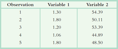
	15-14	Compute the Spearman correlation coefficient for the data listed in Check Your Learning 15-13.
Applying the Concepts	15-15	Here are IQ scores for 10 people: 88, 90, 91, 99, 103, 103, 104, 112, 114, and 139. Why might it be better to use a nonparametric test than a parametric test in this case? Convert the scores for IQ (a scale variable) to ranks (an ordinal variable). What happens to the outlier when the scores are converted from a scale measure to an ordinal measure?
	15-16	Researchers provided accomplishment-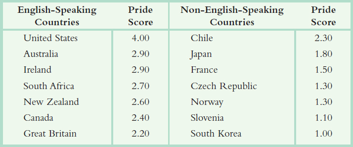related national pride scores for a number of countries (Smith & Kim, 2006). We selected seven countries for which English is the primary language and seven countries for which it is not. We wondered whether English-speaking countries would be different on the variable of accomplishment-related national pride from non-English-speaking countries. The data are in the accompanying table. Conduct a Mann–Whitney U test on these data. Remember to organize the data in one column before starting.

Solutions to these Check Your Learning questions can be found in Appendix D.