nolanessentials3e

6.3 The Central Limit Theorem

139

In the early 1900s, W. S. Gossett discovered how the predictability of the normal curve could improve quality control in the Guinness ale factory. One of the practical problems that Gossett faced was related to sampling yeast cultures: too little yeast led to incomplete fermentation, whereas too much yeast led to a bitter-tasting beer. To test whether he could sample both accurately and economically, Gossett averaged samples of four observations to see how well they represented a known population of 3000 (Gossett, 1908, 1942; Stigler, 1999).

MASTERING THE CONCEPT

6-4: The central limit theorem demonstrates that a distribution made up of the means of many samples (rather than individual scores) approximates a normal curve, even if the underlying population is not normally distributed.

The central limit theorem refers to how a distribution of sample means is a more normal distribution than a distribution of scores, even when the population distribution is not normal.

This small adjustment (taking the average of four samples rather than using just one sample) is possible because of the central limit theorem. The central limit theorem refers to how a distribution of sample means is a more normal distribution than a distribution of scores, even when the population distribution is not normal. Indeed, as sample size increases, a distribution of sample means more closely approximates a normal curve. More specifically, the central limit theorem demonstrates two important principles:

Repeated sampling approximates a normal curve, even when the original population is not normally distributed.
A distribution of means is less variable than a distribution of individual scores.

A distribution of means is a distribution composed of many means that are calculated from all possible samples of a given size, all taken from the same population.

A Distribution of Means A distribution of means reduces the influence of individual outliers such as the length of the fingernails of the woman on the left. When her extreme score is part of a sample that includes smaller, more typical scores, the mean of that sample will be smaller than her individual score. That is why a distribution based on means is less variable than a distribution based on individual scores.

Saovadee/Shutterstock

Instead of randomly sampling a single data point, Gossett randomly sampled four data points from the population of 3000 and computed the average. He did this repeatedly and used those many averages to create a distribution of means. A distribution of means is a distribution composed of many means that are calculated from all possible samples of a given size, all taken from the same population. Put another way, the numbers that make up the distribution of means are not individual scores; they are means of samples of individual scores. Distributions of means are frequently used to understand data across a range of contexts; for example, when a university reports the mean standardized test score of incoming first-year students, that mean would be understood in relation to a distribution of means instead of a distribution of scores.

140

Gossett experimented with using the average of four data points as his sample, but there is nothing magical about the number four. A mean test score for incoming students would have a far larger sample size. The important outcome is that a distribution of means more consistently produces a normal distribution (although with less variance) even when the population distribution is not normal. It might help your understanding to know that the central limit theorem works because a sample of four, for example, will minimize the effect of outliers. When an outlier is just one of four scores being sampled and averaged, the average won’t be as extreme as the outlier.

In this section, we learn how to create a distribution of means, as well as how to calculate a z score for a mean (more accurately called a z statistic when calculated for means rather than scores). We also learn why the central limit theorem indicates that, when conducting hypothesis testing, a distribution of means is more useful than a distribution of scores.

Creating a Distribution of Means

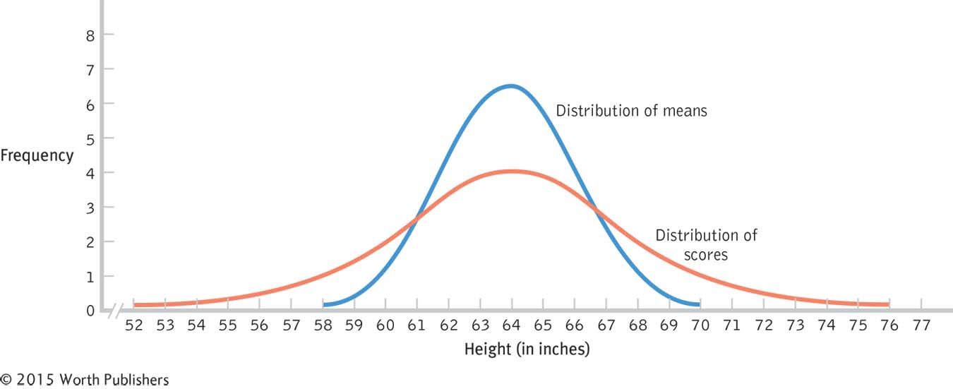
The central limit theorem underlies many statistical processes that are based on a distribution of means. A distribution of means is more tightly clustered (has a smaller standard deviation) than a distribution of scores.

EXAMPLE 6.10

In class, we conduct an exercise with our students that demonstrates the central limit theorem in action. We start by writing the numbers in Table 6-1 on 140 individual index cards that can be mixed together in a hat. The numbers represent the heights, in inches, of 140 college students from the authors’ classes. As before, we treat these 140 students as the entire population.

First, we randomly pull one card at a time and record its score by marking it on a histogram. After recording the score, we return the card to the container representing the population of scores and mix all the cards before pulling the next card. (Not surprisingly, this is known as sampling with replacement.) We continue until we have plotted at least 30 scores, drawing a square for each one so that bars emerge above each value. This creates the beginning of a distribution of scores. Using this method, we created the histogram in Figure 6-10.

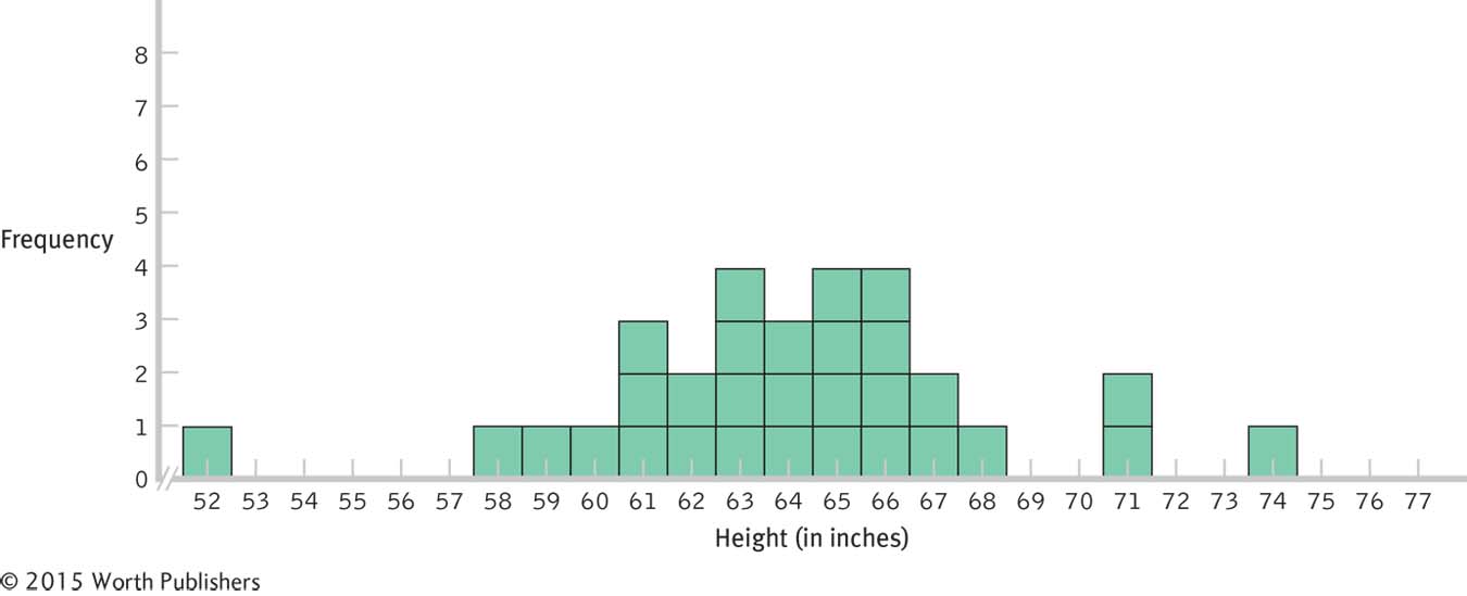Figure 6.11: FIGURE 6-10
Creating a Distribution of Scores
This distribution is one of many that could be created by pulling 30 numbers, one at a time, and replacing the numbers between pulls, from the population of 140 heights. If you create a distribution of scores yourself from these data, it should look roughly bell-shaped like this one—that is, unimodal and symmetric.

141
Now, we randomly pull three cards at a time, compute the mean of these three scores (rounding to the nearest whole number), and record this mean on a different histogram. As before, we draw a square for each mean, with each stack of squares resembling a bar. Again, we return each set of cards to the population and mix before pulling the next set of three. We continue until we have plotted at least 30 values. This is the beginning of a distribution of means. Using this method, we created the histogram in Figure 6-11.

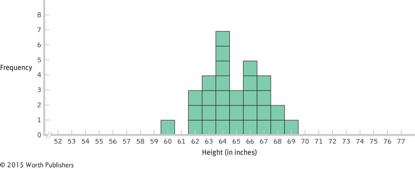Figure 6.12: FIGURE 6-11
Creating a Distribution of Means
Compare this distribution of means to the distribution of scores in Figure 6-10. The mean is the same and it is still roughly bell-shaped. The spread is narrower, however, so there is a smaller standard deviation. This particular distribution is one of many similar distributions that could be created by pulling 30 means (the average of three numbers at a time) from the population of 140 heights.

142

The distribution of scores in Figure 6-10, similar to those we create when we do this exercise in class, ranges from 52 to 77, with a peak in the middle. If we had a larger population, and if we pulled many more numbers, the distribution would become more and more normal. Notice that the distribution is centered roughly around the actual population mean, 64.89. Also notice that all, or nearly all, scores fall within 3 standard deviations of the mean. The population standard deviation of these scores is 4.09. So nearly all scores should fall within this range:

64.89 − 3(4.09) = 52.62 and 64.89 + 3(4.09) = 77.16

In fact, the range of scores—52 through 77—in this population of 140 heights is very close to this range.

Is there anything different about the distribution of means in Figure 6-11? Yes, there are not as many means at the far tails of the distribution as in the distribution of scores—we no longer have any values in the 50s or 70s. However, there are no changes in the center of the distribution. The distribution of means is still centered around the actual mean of 64.89. This makes sense. The means of three scores each come from the same set of scores, so the mean of the individual sample means should be the same as the mean of the whole population of scores.

Why does the spread decrease when we create a distribution of means rather than a distribution of scores? When we plotted individual scores, an extreme score was plotted on the distribution. But when we plotted means, we averaged that extreme score with two other scores. So each time we pulled a score in the 70s, we tended to pull two lower scores as well; when we pulled a score in the 50s, we tended to pull two higher scores as well.

What do you think would happen if we created a distribution of means of 10 scores rather than 3? As you might guess, the distribution would be even narrower because there would be more scores to balance the occasional extreme score. The mean of each set of 10 scores is likely to be even closer to the actual mean of 64.89. What if we created a distribution of means of 100 scores, or of 10,000 scores? The larger the sample size, the smaller the spread of the distribution of means.

Characteristics of the Distribution of Means

Because the distribution of means is less variable than the distribution of scores, the distribution of means needs its own standard deviation—a smaller standard deviation than we used for the distribution of individual scores.

The data presented in Figure 6-12 allow us to visually verify that the distribution of means needs a smaller standard deviation. Using the population mean of 64.886 and standard deviation of 4.086, the z scores for the end scores of 60 and 69 are −1.20 and 1.01, respectively—not even close to 3 standard deviations. These z scores are wrong for this distribution. We need to use a standard deviation of sample means rather than a standard deviation of individual scores.

Figure 6.13: FIGURE 6-12
Using the Appropriate Measure of Spread
Because the distribution of means is narrower than the distribution of scores, it has a smaller standard deviation. This standard deviation has its own name: standard error.

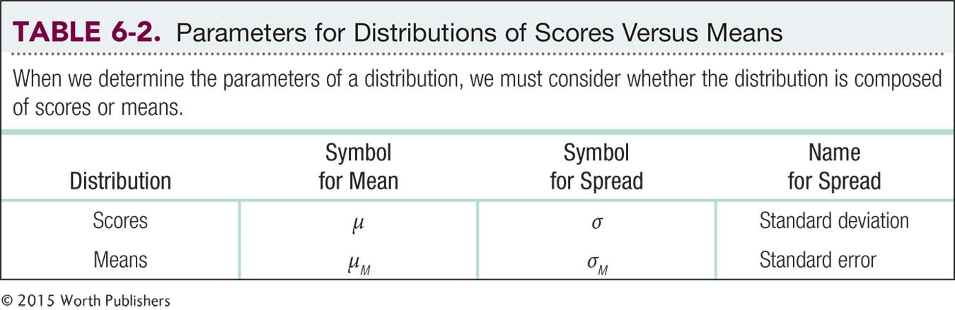
Language Alert! We use slightly modified language and symbols when we describe distributions of means instead of distributions of scores. The mean of a distribution of means is the same as the mean of a population of scores, but it uses the symbol μ_M (pronounced “mew sub em”). The μ indicates that it is the mean of a population, and the subscript M indicates that the population is composed of sample means—the means of all possible samples of a given size from a particular population of individual scores.

MASTERING THE CONCEPT

6-5: A distribution of means has the same mean as a distribution of scores from the same population, but a smaller standard deviation.

143

Standard error is the name for the standard deviation of a distribution of means.

We also need a new symbol and a new name for the standard deviation of the distribution of means—the typical amount that a sample mean varies from the population mean. The symbol is σ_M (pronounced “sigma sub em”). The subscript M again stands for mean; this is the standard deviation of the population of means calculated for all possible samples of a given size. The symbol has its own name: standard error is the name for the standard deviation of a distribution of means. Table 6-2 summarizes the alternative names that describe these related ideas.

MASTERING THE FORMULA

6-3: The formula for standard error is:

We divide the standard deviation for the population by the square root of the sample size.

Fortunately, there is a simple calculation that lets us know exactly how much smaller the standard error, σ_M, is than the standard deviation, σ. As we’ve noted, the larger the sample size, the narrower the distribution of means and the smaller the standard deviation of the distribution of means—the standard error. We calculate the standard error by taking into account the sample size used to calculate the means that make up the distribution. The standard error is the standard deviation of the population divided by the square root of the sample size, N. The formula is:

EXAMPLE 6.11

144

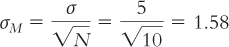
Imagine that the standard deviation of the distribution of individual scores is 5 and we have a sample of 10 people. The standard error would be:

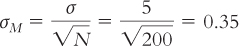
The spread is smaller when we calculate means for samples of 10 people because any extreme scores are balanced by less extreme scores. With a larger sample size of 200, the spread is even smaller because there are many more scores close to the mean to balance out any extreme scores. The standard error would then be:

A distribution of means faithfully obeys the central limit theorem. Even if the population of individual scores is not normally distributed, the distribution of means will approximate the normal curve if the samples are composed of at least 30 scores. The three graphs in Figure 6-13 depict (a) a distribution of individual scores that is extremely skewed in the positive direction, (b) the less skewed distribution that results when we create a distribution of means using samples of 2, and (c) the approximately normal curve that results when we create a distribution of means using samples of 25. We have learned three important characteristics of the distribution of means:

Figure 6.15: FIGURE 6-13
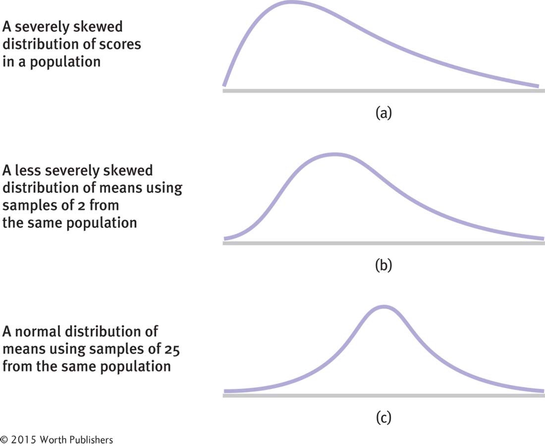
The Mathematical Magic of Large Samples
Even with a population of individual scores that are not normally distributed, the distribution of means approximates a normal curve as the sample gets larger.

As sample size increases, the mean of a distribution of means remains the same.

145
The standard deviation of a distribution of means (called the standard error) is smaller than the standard deviation of a distribution of scores. As sample size increases, the standard error becomes ever smaller.
The shape of the distribution of means approximates the normal curve if the distribution of the population of individual scores has a normal shape or if the size of each sample that makes up the distribution is at least 30 (the central limit theorem).

Using the Central Limit Theorem to Make Comparisons with z Scores

MASTERING THE FORMULA

6-4: The formula for z based on the mean of a sample is:

We subtract the mean of the distribution of means from the mean of the sample, then we divide by the standard error, the standard deviation of the distribution of means.

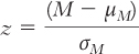
z scores are a standardized version of raw scores based on the population. But we seldom have the entire population to work with, so we typically calculate the mean of a sample and calculate a z score based on a distribution of means. When we calculate the z score, we simply use a distribution of means instead of a distribution of scores. The z formula changes only in the symbols it uses:

Note that we now use M instead of X because we are calculating a z score for a sample mean rather than for an individual score. Because the z score now represents a mean, not an actual score, it is often referred to as a z statistic. Specifically, the z statistic tells us how many standard errors a sample mean is from the population mean.

EXAMPLE 6.12

Let’s consider a distribution for which we know the population mean and standard deviation. Several hundred universities reported data from their counseling centers (Gallagher, 2009). (For this example, we’ll treat this sample as the entire population of interest.) The study found that an average of 8.5 students per institution were hospitalized for mental illness over 1 year. For the purposes of this example, we’ll assume a standard deviation of 3.8. Let’s say we develop a prevention program to reduce the numbers of hospitalizations and we recruit 30 universities to participate. After 1 year, we calculate a mean of 7.1 hospitalizations at these 30 institutions. Is this an extreme sample mean, given the population?

To find out, let’s imagine the distribution of means for samples of 30 hospitalization scores. We would collect the means the same way we collected the means of three heights in the earlier example—just with far more means. The average of all those means would have the same mean as the population but the spread would be narrower. The spread of the distribution is skinnier because any extreme hospitalization scores would now be part of a sample that likely included less extreme scores. So, the mean for each sample is less likely to be extreme than is an individual score. The distribution of all of these means, then, would be less variable than the distribution of scores. Here are the mean and standard error of the sample of universities, using proper symbolic notation:

μ_M = μ = 8.5

146

At this point, we have all the information we need to calculate the z statistic:

From this z statistic, we could determine how extreme the mean number of hospitalizations is in terms of a percentage. Then we could draw a conclusion about whether we would be likely to find a mean number of hospitalizations of 7.1 in a sample of 30 universities if the prevention program did not work. The useful combination of a distribution of means and a z statistic has led us to a point where we’re prepared for inferential statistics and hypothesis testing.

CHECK YOUR LEARNING

Reviewing the Concepts

According to the central limit theorem, a distribution of sample means based on 30 or more scores approximates the normal distribution, even if the original population is not normally distributed.
A distribution of scores has the same mean as a distribution of means. However, a distribution of scores contains more extreme scores and a larger standard deviation than a distribution of means; this is another principle of the central limit theorem.
z scores may be calculated from a distribution of scores or from a distribution of means. When we calculate a z score for a mean, we usually call it a z statistic.
For the measure of spread, the two calculations use different terms: standard deviation for a distribution of scores and standard error for a distribution of means.
Just as with z scores, the z statistic tells us about the relative position of a mean within a distribution; this can be expressed as a percentile.

Clarifying the Concepts

6-10

What are the main ideas behind the central limit theorem?

6-11

Explain what a distribution of means is.

Calculating the Statistics

6-12

The mean of a distribution of scores is 57, with a standard deviation of 11. Calculate the standard error for a distribution of means based on samples of 35 people.

Applying the Concepts

6-13

Let’s return to the selection of 30 CFC scores that we considered in Check Your Learning 6-2(b):

3.5	3.5	3.0	4.0	2.0	4.0	2.0	4.0	3.5	4.5
4.5	4.0	3.5	2.5	3.5	3.5	4.0	3.0	3.0	2.5
3.0	3.5	4.0	3.5	3.5	2.0	3.5	3.0	3.0	2.5

What is the range of these scores?
Take three means of 10 scores each from this sample of scores, one for each row. What is the range of these means?
Why is the range smaller for the means of samples of 10 scores than for the individual scores themselves?
The mean of these 30 scores is 3.32. The standard deviation is 0.69. Using symbolic notation and formulas (where appropriate), determine the mean and standard error of the distribution of means computed from samples of 10.

Solutions to these Check Your Learning questions can be found in Appendix D.