10.2 Beyond Hypothesis Testing
The APA encourages the use of confidence intervals and effect sizes (as with the z test and the single-
MASTERING THE CONCEPT
10.3: As we can with a z test and a single-
251
Calculating a Confidence Interval for a Paired-Samples t Test
Let’s start by determining the confidence interval for the productivity example.
EXAMPLE 10.2
First, let’s recap the information we need. The population mean difference according to the null hypothesis was 0, and we used the sample to estimate the population standard deviation to be 4.301 and the standard error to be 1.924. The five participants in the study sample had a mean difference of −11. We will calculate the 95% confidence interval around the sample mean difference of −11.
STEP 1: Draw a picture of a t distribution that includes the confidence interval.
We draw a normal curve (Figure 10-4) that has the sample mean difference, −11, at its center instead of the population mean difference, 0.
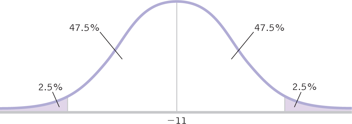
Figure 10-
STEP 2: Indicate the bounds of the confidence interval on the drawing.
As before, 47.5% fall on each side of the mean between the mean and the cutoff, and 2.5% fall in each tail.
STEP 3: Add the critical t statistics to the curve.
For a two-
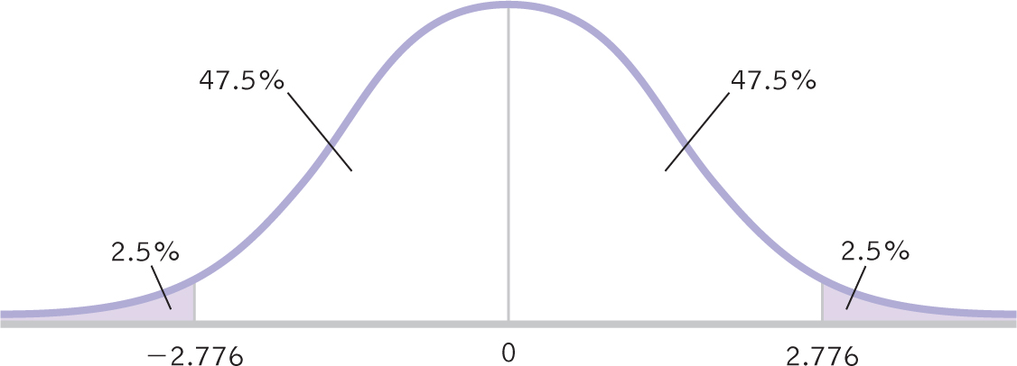
Figure 10-
STEP 4: Convert the critical t statistics back into raw mean differences.
As we do with other confidence intervals, we use the sample mean difference (−11) in the calculations and the standard error (1.924) as the measure of spread. We use the same formulas as for the single-
252
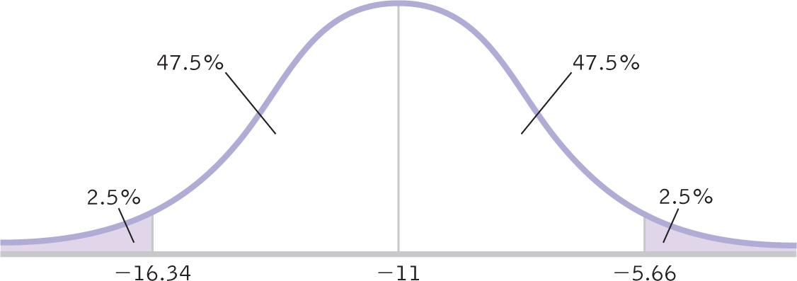
Figure 10-
MASTERING THE FORMULA
10-
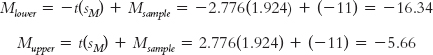
The 95% confidence interval, reported in brackets as is typical, is [−16.34, −5.66].
STEP 5: Verify that the confidence interval makes sense.
The sample mean difference should fall exactly in the middle of the two ends of the interval.
−11 − (−16.34) = 5.34 and −11 − (−5.66) = −5.34
We have a match. The confidence interval ranges from 5.34 below the sample mean difference to 5.34 above the sample mean difference. If we were to sample five people from the same population over and over, the 95% confidence interval would include the population mean 95% of the time. Note that the population mean difference according to the null hypothesis, 0, does not fall within this interval. This means it is not plausible that the difference between those using the 15-
As with other hypothesis tests, the conclusions from both the paired-
Calculating Effect Size for a Paired-Samples t Test
As with a z test, we can calculate the effect size (Cohen’s d) for a paired-
EXAMPLE 10.3
Let’s calculate the effect size for the computer monitor study. Again, we simply use the formula for the t statistic, substituting s for sM (and μ for μM, even though these means are always the same). This means we use 4.301 instead of 1.924 in the denominator. Cohen’s d is now based on the spread of the distribution of individual differences between scores, rather than the distribution of mean differences.
MASTERING THE FORMULA
10- It is the same formula as for the single-
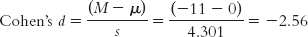
The effect size, d = −2.56, tells us that the sample mean difference and the population mean difference are 2.56 standard deviations apart. This is a large effect. Recall that the sign has no effect on the size of an effect: −2.56 and 2.56 are equivalent effect sizes. We can add the effect size when we report the statistics as follows: t(4) = −5.72, p < 0.05, d = −2.56.
253
Next Steps
Order Effects and Counterbalancing
Order effects refer to how a participant’s behavior changes when the dependent variable is presented for a second time, sometimes called practice effects.
There are particular problems that can occur with a within-
Counterbalancing minimizes order effects by varying the order of presentation of different levels of the independent variable from one participant to the next.
Fortunately, we can limit the confounding influence of order effects. Counterbalancing minimizes order effects by varying the order of presentation of different levels of the independent variable from one participant to the next. For example, half of the participants could be randomly assigned to complete the tasks on the 15-
There are other ways to reduce order effects. In the computer monitor example, we might decide to use a different set of tasks in each testing condition. The order in which the two different sets of tasks are given could be counterbalanced along with the order in which participants are assigned to the two different-

© Amazing Images/Alamy
254
CHECK YOUR LEARNING
Reviewing the Concepts
- We can calculate a confidence interval for a paired-
samples t test. This provides us with an interval estimate rather than simply a point estimate. If 0 is not in the confidence interval, then it is not plausible that there is no difference between the sample and population mean differences. - We also can calculate an effect size (Cohen’s d) for a paired-
samples t test. - Order effects occur when participants’ behavior is affected when a dependent variable is presented a second time.
- Order effects can be reduced through counterbalancing, a procedure in which the different levels of the independent variable are presented in different orders from one participant to the next.
Clarifying the Concepts
- 10-
5 How does creating a confidence interval for a paired-samples t test give us the same information as hypothesis testing with a paired- samples t test? - 10-
6 How do we calculate Cohen’s d for a paired-samples t test?
Calculating the Statistics
- 10-
7 Assume that researchers asked five participants to rate their mood on a scale from 1 to 7 (1 being lowest, 7 being highest) before and after watching a funny video clip. The researchers reported that the average difference between the “before” mood score and the “after” mood score was M = 1.0, s = 1.225. They calculated a paired-samples t test, t(4) = 1.13, p > 0.05 and, using a two- tailed test with a p level of 0.05, failed to reject the null hypothesis. - Calculate the 95% confidence interval for this t test and describe how it results in the same conclusion as the hypothesis test.
- Calculate and interpret Cohen’s d.
Applying the Concepts
- 10-
8 Using the energy-level data presented in Check Your Learning 10- 3 and 10- 4, let’s go beyond hypothesis testing. - Calculate the 95% confidence interval and describe how it results in the same conclusion as the hypothesis test.
- Calculate and interpret Cohen’s d.
Solutions to these Check Your Learning questions can be found in Appendix D.