11.2 Beyond Hypothesis Testing
After working at Guinness, Stella Cunliffe was hired by the British government’s criminology department. She noticed that adult male prisoners who had short prison sentences returned to prison at a very high rate—
MASTERING THE CONCEPT
11.2: As we can with the z test, the single-
Two ways that researchers can evaluate the findings of a hypothesis test are by calculating a confidence interval and an effect size.
Calculating a Confidence Interval for an Independent-Samples t Test
Confidence intervals for the independent-
We use the formula for the independent-
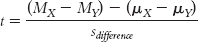
We replace the population mean difference, (μX − μY), with the sample mean difference, (MX − MY)sample, because this is what the confidence interval is centered around. We also indicate that the first mean difference in the numerator refers to the bounds of the confidence intervals, the upper bound in this case:
MASTERING THE FORMULA
![]()
![]() 11-
11-
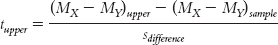
With algebra, we isolate the upper bound of the confidence interval to create the following formula:
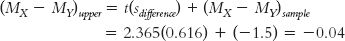
(MX − MY)upper = t(sdifference) + (MX − MY)sample
We create the formula for the lower bound of the confidence interval in exactly the same way, using the negative version of the t statistic:
(MX − MY)lower = −t(sdifference) + (MX − MY)sample
EXAMPLE 11.3
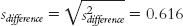
Let’s calculate the confidence interval that parallels the hypothesis test we conducted earlier, comparing ratings of those who are told they are drinking wine from a $10 bottle and ratings of those told they are drinking wine from a $90 bottle (Plassmann et al., 2008). The difference between the means of these samples was calculated in the numerator of the t statistic. It is: 2.5 − 4.0 = −1.5. (Note that the order of subtraction in calculating the difference between means is irrelevant; we could just as easily have subtracted 2.5 from 4.0 and gotten a positive result, 1.5.) The standard error for the differences between means, sdifference was calculated to be 0.616. The degrees of freedom were determined to be 7. Here are the five steps for determining a confidence interval for a difference between means:
273
STEP 1: Draw a normal curve with the sample difference between means in the center (as shown in Figure 11-4).
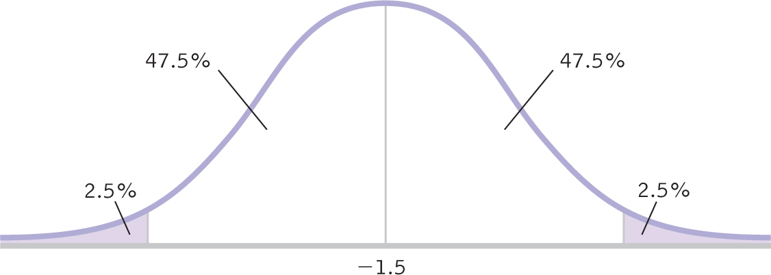
Figure 11-
STEP 2: Indicate the bounds of the confidence interval on either end, and write the percentages under each segment of the curve.
(See Figure 11-4.)
STEP 3: Look up the t statistics for the lower and upper ends of the confidence interval in the t table.
Use a two-
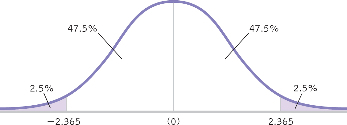
Figure 11-
STEP 4: Convert the t statistics to raw differences between means for the lower and upper ends of the confidence interval.
For the lower end, the formula is:
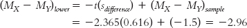
274
For the upper end, the formula is:
The confidence interval is [−2.96, −0.04], as shown in Figure 11-6.
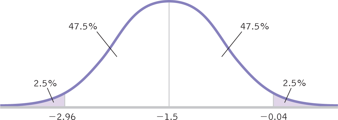
Figure 11-
STEP 5: Check your answer.
Each end of the confidence interval should be exactly the same distance from the sample mean.
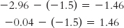
The interval checks out. The bounds of the confidence interval are calculated as the difference between sample means, plus or minus 1.46.
Also, the confidence interval does not include 0. Thus, it is not plausible that there is no difference between means. We can conclude that people told they are drinking wine from a $10 bottle give different ratings, on average, than those told they are drinking wine from a $90 bottle.
When we conducted the independent-
Calculating Effect Size for an Independent-Samples t Test
EXAMPLE 11.4
As with all hypothesis tests, it is recommended that the results be supplemented with an effect size. For an independent-
Stage (a) (variance for each sample):
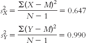
275
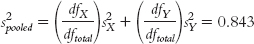
Stage (b) (combining variances):
Stage (c) (variance form of standard error for each sample):
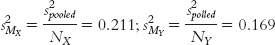
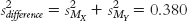
Stage (d) (combining variance forms of standard error):
Stage (e) (converting the variance form of standard error to the standard deviation form of standard error):
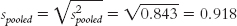
Because the goal is to disregard the influence of sample size in order to calculate Cohen’s d, we want to use the standard deviation, rather than the standard error, in the denominator. So we can ignore the last three stages, all of which contribute to the calculation of standard error. That leaves stages (a) and (b). It makes more sense to use the one that includes information from both samples, so we focus our attention on stage (b). Here is where many students make a mistake. What we have calculated in stage (b) is pooled variance, not pooled standard deviation. We must take the square root of the pooled variance to get the pooled standard deviation, the appropriate value for the denominator of Cohen’s d.
The test statistic that we calculated for this study was:
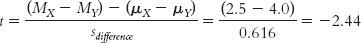
For Cohen’s d, we simply replace the denominator with standard deviation, spooled, instead of standard error, sdifference.
MASTERING THE FORMULA
11-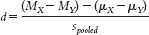 . The formula is similar to that for the test statistic in an independent-
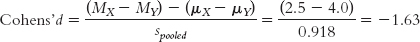
For this study, the effect size is reported as: d = −1.63. The two sample means are 1.63 standard deviations apart. According to the conventions shown again in Table 11-2, we learned in Chapter 8 (0.2 is a small effect; 0.5 is a medium effect; 0.8 is a large effect), this is a large effect.
| Effect Size | Convention | Overlap |
|---|---|---|
| Small | 0.2 | 85% |
| Medium | 0.5 | 67% |
| Large | 0.8 | 53% |
276
Next Steps
Data Transformations
When we conduct hypothesis tests, such as the independent-
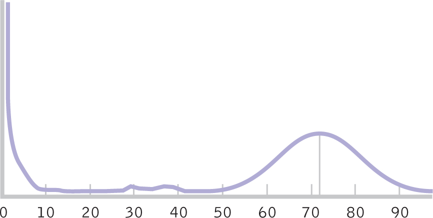
Figure 11-
In a situation such as the childhood mortality data, we can transform skewed data into a more normal distribution. In fact, even when the sample is small and the population distribution is skewed, there are still a variety of ways for us to transform skewed data so that they are no longer skewed. One way is to transform scale data to ordinal data. For example, consider a sample of incomes of $24,000, $27,000, $35,000, $46,000, and $550,000. Here, the income of $550,000 is far higher than the next-
| Scale: | $24,000 $27,000 $35,000 $46,000 $550,000 |
| Ordinal: | 5 4 3 2 1 |
Now $550,000 is ranked first and $46,000 is ranked second. However, the large difference between the two scores disappeared when we transformed the data from a scale measure to an ordinal measure. The problem with transforming scale data to ordinal data is that a z test or a t test only works with scale data. (We will learn tests we can use with ordinal data in Chapters 17 and 18.) Fortunately, other transformations also can diminish skew while still allowing us to use the more powerful parametric tests we’ve learned so far.
A square root transformation reduces skew by compressing both the negative and positive sides of a skewed distribution.
A square root transformation reduces skew by compressing both the negative and positive sides of a skewed distribution. Let’s take the same five incomes on a scale measure, but instead of converting them to ranks, we’ll take the square root of each of them. As we will see, the effect is more dramatic on the higher values.
| Scale: | $24,000 $27,000 $35,000 $46,000 $550,000 |
| Square root: | $154.92 $164.32 $187.08 $214.48 $741.62 |
Now the severe outlier of $550,000, much higher than the next-
277
Here we have discussed two ways to deal with skewed data:
- Transform a scale variable to an ordinal variable.
- Use a data transformation such as square root transformation to “squeeze” the data together to make them more normal.
Remember that we need to apply any kind of data transformation to every observation in the data set. Furthermore, data transformation should only be used if it isn’t possible to operationalize the variable of interest in a better way. You want to keep your statistical analyses as simple as possible and no simpler.
CHECK YOUR LEARNING
Reviewing the Concepts
- A confidence interval can be created with a t distribution around a difference between means.
- We can calculate an effect size, Cohen’s d, for an independent-
samples t test. - When the sample data suggest that the underlying population distribution is not normal and the sample size is small, it is sometimes possible to use data transformation to transform skewed data into a more normal distribution.
Clarifying the Concepts
- 11-
5 Why do we calculate confidence intervals? - 11-
6 How does considering the conclusions in terms of effect size help to prevent incorrect interpretations of the findings?
Calculating the Statistics
- 11-
7 Use the hypothetical data on level of agreement with a supervisor, as listed here, to calculate the following. We already made some of these calculations for Check Your Learning 11-3. - Group 1 (low trust in leader): 3, 2, 4, 6, 1, 2
- Group 2 (high trust in leader): 5, 4, 6, 2, 6
- Calculate the 95% confidence interval.
- Calculate effect size using Cohen’s d.
Applying the Concepts
- 11-
8 Explain what the confidence interval calculated in Check Your Learning 11-7 tells us. Why is this confidence interval superior to the hypothesis test that we conducted? - 11-
9 Interpret the meaning of the effect size calculated in Check Your Learning 11-7. What does this add to the confidence interval and hypothesis test?
Solutions to these Check Your Learning questions can be found in Appendix D.