14.3 Conducting a Two-Way Between-Groups ANOVA
Advertising agencies understand that interactions can help them target their advertising campaigns. For example, researchers demonstrated that an increased exposure to dogs (linked in our memories to cats through familiar phrases such as “it’s raining cats and dogs”) positively influenced people’s evaluations of Puma sneakers (a brand whose name refers to a cat), but only for people who recognized the Puma logo (Berger & Fitzsimons, 2008). The interaction between frequency of exposure to dogs (one independent variable) and whether or not someone could recognize the Puma logo (a second independent variable) combined to create a more positive evaluation of Puma sneakers (the dependent variable). Once again, both independent variables were needed to produce an interaction.
365
Behavioral scientists explore interactions by using two-
The three ideas being tested in a two-
The Six Steps of Two-Way ANOVA
Two-
EXAMPLE 14.4
Does myth busting really improve public health? Here are some myths and facts.
From the Web site of the Headquarters Counseling Center (2005) in Lawrence,
Kansas:
- Myth: “Suicide happens without warning.”
- Fact: “Most suicidal persons talk about and/or give behavioral clues about their suicidal feelings, thoughts, and intentions.”
From the Web site for the World Health Organization (2007):
- Myth: “Disasters bring out the worst in human behavior.”
- Fact: “Although isolated cases of antisocial behavior exist, the majority of people respond spontaneously and generously.”
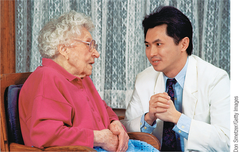
A group of Canadian researchers examined the effectiveness of myth busting (Skurnik, Yoon, Park, & Schwarz, 2005). They wondered whether the effectiveness of debunking false medical claims depends on the age of the person targeted by the message. In one study, they compared two groups of adults: younger adults, ages 18–
366
The two independent variables in this study were age, with two levels (younger, older), and number of repetitions, with two levels (once, three times). The dependent variable, proportion of responses that were wrong after a 3-
| Experimental Conditions | Proportion of Responses That Were Wrong | Mean |
|---|---|---|
| Younger, one repetition | 0.25, 0.21, 0.14 | 0.20 |
| Younger, three repetitions | 0.07, 0.13, 0.16 | 0.12 |
| Older, one repetition | 0.27, 0.22, 0.17 | 0.22 |
| Older, three repetitions | 0.33, 0.31, 0.26 | 0.30 |
Let’s consider the steps of hypothesis testing for a two-
STEP 1: Identify the populations, distribution, and assumptions.
The first step of hypothesis testing for a two-
| One Repetition (1) | Three Repetitions (3) | |
|---|---|---|
| Younger (Y) | Y; 1 | Y; 3 |
| Older (O) | O; 1 | O; 3 |
There are four populations, each with labels representing the levels of the two independent variables to which they belong.
- Population 1 (Y; 1): Younger adults who hear one repetition of a false claim.
- Population 2 (Y; 3): Younger adults who hear three repetitions of a false claim.
- Population 3 (O; 1): Older adults who hear one repetition of a false claim.
- Population 4 (O; 3): Older adults who hear three repetitions of a false claim.
We next consider the characteristics of the data to determine the distributions to which we compare the sample. We have more than two groups, so we need to consider variances to analyze differences among means. Therefore, we use F distributions.
367
Finally, we list the hypothesis test that we use for those distributions and check the assumptions for that test. For F distributions, we use ANOVA—
The assumptions are the same for all types of ANOVA. The sample should be selected randomly; the populations should be distributed normally; and the population variances should be equal. Let’s explore that a bit further.
(1) These data were not randomly selected. Younger adults were recruited from a university, and older adults were recruited from the local community. Because random sampling was not used, we must be cautious when generalizing from these samples. (2) The researchers did not report whether they investigated the shapes of the distributions of their samples to assess the shapes of the underlying populations. (3) The researchers did not provide standard deviations of the samples as an indication of whether the population spreads might be approximately equal—
Summary: Population 1 (Y; 1): Younger adults who hear one repetition of a false claim. Population 2 (Y; 3): Younger adults who hear three repetitions of a false claim. Population 3 (O; 1): Older adults who hear one repetition of a false claim. Population 4 (O; 3): Older adults who hear three repetitions of a false claim.
The comparison distributions will be F distributions. The hypothesis test will be a two-
STEP 2: State the null and research hypotheses.
The second step, to state the null and research hypotheses, is similar to that for a one-
The hypotheses for the interaction are typically stated in words but not in symbols. The null hypothesis is that the effect of one independent variable is not dependent on the levels of the other independent variable. The research hypothesis is that the effect of one independent variable depends on the levels of the other independent variable. It does not matter which independent variable we list first (e.g., “the effect of age is not dependent…” or “the effect of number of repetitions is not dependent…”). Write the hypotheses in the way that makes the most sense to you.
Summary: The hypotheses for the main effect of the first independent variable, age, are as follows. Null hypothesis: On average, compared with older adults, younger adults have the same proportion of responses that are wrong when remembering which claims are myths—
368
The hypotheses for the main effect of the second independent variable, number of repetitions, are as follows. Null hypothesis: On average, those who hear one repetition have the same proportion of responses that are wrong when remembering which claims are myths compared with those who hear three repetitions—
The hypotheses for the interaction of age and number of repetitions are as follows. Null hypothesis: The effect of number of repetitions is not dependent on the levels of age. Research hypothesis: The effect of number of repetitions depends on the levels of age.
STEP 3: Determine the characteristics of the comparison distribution.
The third step is similar to that of a one-
MASTERING THE FORMULA
![]() 14-
14-
MASTERING THE FORMULA
![]() 14-
14-
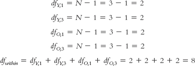
For each main effect, the between-
dfrows(age) = Nrows − 1 = 2 − 1 = 1
The second independent variable, number of repetitions, is in the columns of the table of cells, so the between-
dfcolumns(reps) = Ncolumns − 1 = 2 − 1 = 1
MASTERING THE FORMULA
14-
We now need a between-
dfinteraction = (dfrows(age))(dfcolumns(reps)) = (1)(1) = 1
The within-
MASTERING THE FORMULA
![]() 14-
14-
369
For a check on our work, we calculate the total degrees of freedom just as we did for the one-
MASTERING THE FORMULA
14-
dftotal = Ntotal − 1 = 12 − 1 = 11
We now add up the three between-
11 = 1 + 1 + 1 + 8
Finally, for this step, we list the distributions with their degrees of freedom for the three effects. Note that, although the between-
Summary: Main effect of age: F distribution with 1 and 8 degrees of freedom. Main effect of number of repetitions: F distribution with 1 and 8 degrees of freedom. Interaction of age and number of repetitions: F distribution with 1 and 8 degrees of freedom. (Note: It is helpful to include all degrees of freedom calculations in this step.)
STEP 4: Determine the critical values, or cutoffs.
Again, this step for the two-
For each main effect and for the interaction, we look up the within-
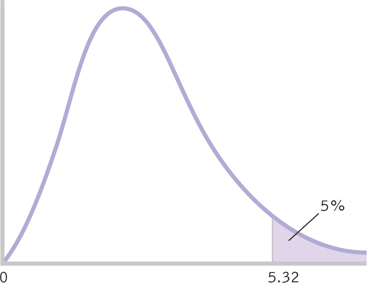
Figure 14-
Summary: There are three critical values (which in this case are all the same), as seen in the curve in Figure 14-8. The critical F value for the main effect of age is 5.32. The critical F value for the main effect of number of repetitions is 5.32. The critical F value for the interaction of age and number of repetitions is 5.32.
STEP 5: Calculate the test statistic.
As with the one-
370
STEP 6: Make a decision.
This step is the same as for a one-
First, if we are able to reject the null hypothesis for the interaction, then we draw a specific conclusion with the help of a table and graph. Because we have more than two groups, we use a post hoc test, such as the one that we learned in Chapter 12. When there are three effects, post hoc tests are typically implemented separately for each main effect and for the interaction (Hays, 1994). If the interaction is statistically significant, then it might not matter whether the main effects are also significant; if they are also significant, then those findings are usually qualified by the interaction, and are not described separately. The overall pattern of cell means tells the whole story.
Second, if we are not able to reject the null hypothesis for the interaction, then we focus on any significant main effects, drawing a specific directional conclusion for each. In this study, each independent variable has only two levels, so there is no need for a post hoc test. If there were three or more levels, however, then each significant main effect would require a post hoc test to determine exactly where the differences lie. Third, if we do not reject the null hypothesis for either main effect or the interaction, then we can only conclude that there is insufficient evidence from this study to support the research hypotheses. We will complete step 6 of hypothesis testing for this study in the next section, after we consider the calculations of the source table for a two-
Identifying Four Sources of Variability in a Two-Way ANOVA
In this section, we complete step 5 for a two-
MASTERING THE FORMULA
![]() 14-
14-
First, we calculate the total sum of squares (Table 14-13). We calculate this number in exactly the same way as we do for a one-
SStotal = Σ(X − GM)2 = 0.0672
| X | X − GM | (X − GM)2 | |
|---|---|---|---|
| Y, 1 | 0.25 | (0.25 − 0.21) = 0.04 | 0.0016 |
| 0.21 | (0.21 − 0.21) = 0.00 | 0.0000 | |
| 0.14 | (0.14 − 0.21) = 20.07 | 0.0049 | |
| Y, 3 | 0.07 | (0.07 − 0.21) = 20.14 | 0.0196 |
| 0.13 | (0.13 − 0.21) = 20.08 | 0.0064 | |
| 0.16 | (0.16 − 0.21) = 20.05 | 0.0025 | |
| 0, 1 | 0.27 | (0.27 − 0.21) = 0.06 | 0.0036 |
| 0.22 | (0.22 − 0.21) = 0.01 | 0.0001 | |
| 0.17 | (0.17 − 0.21) = 20.04 | 0.0016 | |
| 0, 3 | 0.33 | (0.33 − 0.21) = 0.12 | 0.0144 |
| 0.31 | (0.31 − 0.21) = 0.10 | 0.0100 | |
| 0.26 | (0.26 − 0.21) = 0.05 | 0.0025 |
371
MASTERING THE FORMULA
![]() 14-
14-
We now calculate the between-
SSbetween(rows) = Σ(Mrow(age) − GM)2 = 0.03
| One Repetition (1) | Three Repetitions (3) | ||
|---|---|---|---|
| Younger (Y) | 0.20 | 0.12 | 0.16 |
| Older (O) | 0.22 | 0.30 | 0.26 |
| 0.21 | 0.21 | 0.21 |
| X | Mrow(age) − GM | (Mrow(age) − GM)2 | |
|---|---|---|---|
| Y, 1 | 0.25 | (0.16 − 0.21) = 20.05 | 0.0025 |
| 0.21 | (0.16 − 0.21) = 20.05 | 0.0025 | |
| 0.14 | (0.16 − 0.21) = 20.05 | 0.0025 | |
| Y, 3 | 0.07 | (0.16 − 0.21) = 20.05 | 0.0025 |
| 0.13 | (0.16 − 0.21) = 20.05 | 0.0025 | |
| 0.16 | (0.16 − 0.21) = 20.05 | 0.0025 | |
| O, 1 | 0.27 | (0.26 − 0.21) = 0.05 | 0.0025 |
| 0.22 | (0.26 − 0.21) = 0.05 | 0.0025 | |
| 0.17 | (0.26 − 0.21) = 0.05 | 0.0025 | |
| O, 3 | 0.33 | (0.26 − 0.21) = 0.05 | 0.0025 |
| 0.31 | (0.26 − 0.21) = 0.05 | 0.0025 | |
| 0.26 | (0.26 − 0.21) = 0.05 | 0.0025 |
372
MASTERING THE FORMULA
![]() 14-
14-
We repeat this process for the second possible main effect, that of the independent variable in the columns (Table 14-16). The between-
SSbetween(columns) = Σ(Mcolumn(reps) − GM)2 = 0
| X | Mcolumn(reps) − GM | (Mcolumn(reps) − GM)2 | |
|---|---|---|---|
| Y, 1 | 0.25 | (0.21 − 0.21) = 0 | 0 |
| 0.21 | (0.21 − 0.21) = 0 | 0 | |
| 0.14 | (0.21 − 0.21) = 0 | 0 | |
| Y, 3 | 0.07 | (0.21 − 0.21) = 0 | 0 |
| 0.13 | (0.21 − 0.21) = 0 | 0 | |
| 0.16 | (0.21 − 0.21) = 0 | 0 | |
| O, 1 | 0.27 | (0.21 − 0.21) = 0 | 0 |
| 0.22 | (0.21 − 0.21) = 0 | 0 | |
| 0.17 | (0.21 − 0.21) = 0 | 0 | |
| O, 3 | 0.33 | (0.21 − 0.21) = 0 | 0 |
| 0.31 | (0.21 − 0.21) = 0 | 0 | |
| 0.26 | (0.21 − 0.21) = 0 | 0 |
MASTERING THE FORMULA
![]() 14-
14-
The within-
SSwithin = Σ(X − Mcell)2 = 0.018
| X | ∑(X − Mcell) | ∑(X − Mcell)2 | |
|---|---|---|---|
| Y, 1 | 0.25 | (0.25 − 0.20) = 0.05 | 0.0025 |
| 0.21 | (0.21 − 0.20) = 0.01 | 0.0001 | |
| 0.14 | (0.14 − 0.20) = 20.06 | 0.0036 | |
| Y, 3 | 0.07 | (0.07 − 0.12) = 20.05 | 0.0025 |
| 0.13 | (0.13 − 0.12) = 0.01 | 0.0001 | |
| 0.16 | (0.16 − 0.12) = 0.04 | 0.0016 | |
| O, 1 | 0.27 | (0.27 − 0.22) = 0.05 | 0.0025 |
| 0.22 | (0.22 − 0.22) = 0.00 | 0.0000 | |
| 0.17 | (0.17 − 0.22) = 20.05 | 0.0025 | |
| O, 3 | 0.33 | (0.33 − 0.30) = 0.03 | 0.0009 |
| 0.31 | (0.31 − 0.30) = 0.01 | 0.0001 | |
| 0.26 | (0.26 − 0.30) = 20.04 | 0.0016 |
MASTERING THE FORMULA
![]() 14-
14-
All we need now is the between-
373
SSbetween(interaction) =
SStotal − (SSbetween(rows) + SSbetween(columns) + SSwithin)
The calculations are:
MASTERING THE FORMULA
![]() 14-
14-
SSbetween(interaction) = 0.0672 − (0.03 + 0 + 0.018) = 0.0192
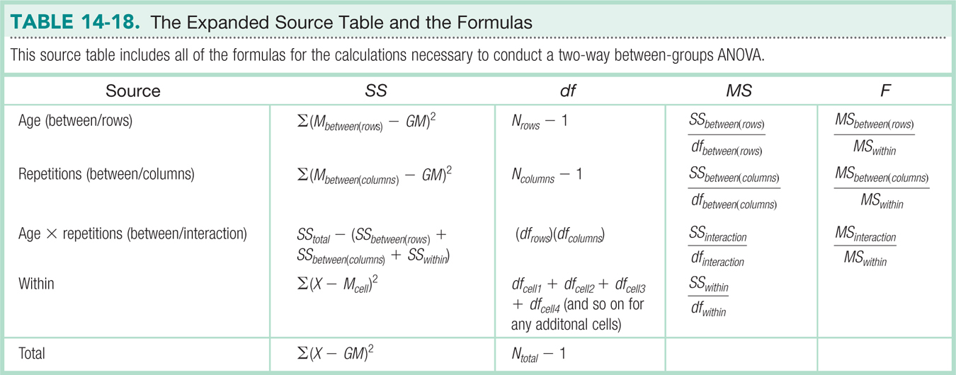
Now we complete step 6 of hypothesis testing by calculating the F statistics using the formulas in Table 14-18. The results are in the source table (Table 14-19). The main effect of age is statistically significant because the F statistic, 13.04, is larger than the critical value of 5.32. The means tell us that older participants tend to make more mistakes, remembering more medical myths as true, than do younger participants. The main effect of number of repetitions is not statistically significant, however, because the F statistic of 0.00 is not larger than the cutoff of 5.32. It is unusual to have an F statistic of 0.00. Even when there is no statistically significant effect, there is usually some difference among means due to random sampling. The interaction is also statistically significant because the F statistic of 8.35 is larger than the cutoff of 5.32. Therefore, we construct a bar graph of the cell means, as seen in Figure 14-9, to interpret the interaction.
| Source | SS | df | MS | F |
|---|---|---|---|---|
| Age (A) | 0.0300 | 1 | 0.0300 | 13.04 |
| Repetitions (R) | 0.0000 | 1 | 0.0000 | 0.00 |
| A × R | 0.0192 | 1 | 0.0192 | 8.35 |
| Within | 0.0180 | 8 | 0.0023 | |
| Total | 0.0672 | 11 |
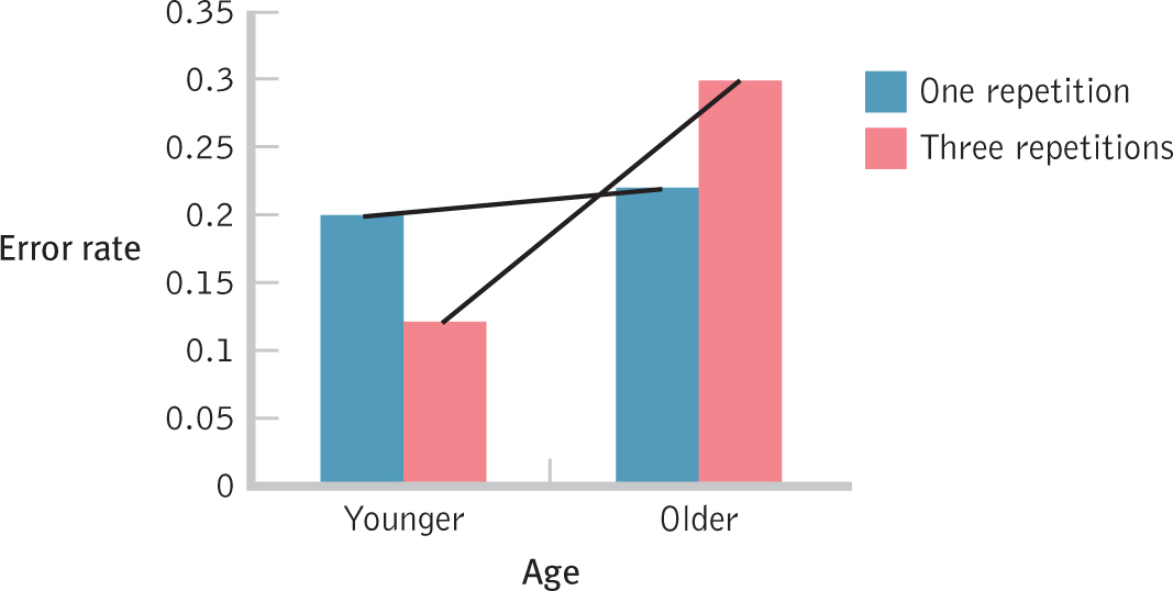
Figure 14-
In Figure 14-9, the lines are not parallel; in fact, they intersect without even having to extend them beyond the graph. We see that among younger participants, the proportion of responses that were incorrect was lower, on average, with three repetitions than with one repetition. Among older participants, the proportion of responses that were incorrect was higher, on average, with three repetitions than with one repetition. Does repetition help? It depends. It helps for younger people but is detrimental for older people. Specifically, repetition tends to help younger people distinguish between myth and fact. But the mere repetition of a medical myth tends to lead older people to be more likely to view it as fact. The researchers speculate that older people remember that they are familiar with a statement but forget the context in which they heard it. Because the direction of the effect of repetition reverses from one age group to another, this is a qualitative interaction.
374
Effect Size for Two-Way ANOVA
With a two-
375
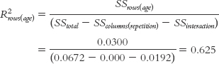
For the first main effect, the one in the rows of the table of cells, the formula is:
MASTERING THE FORMULA
![]() 14-
14-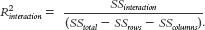 .
.
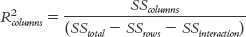
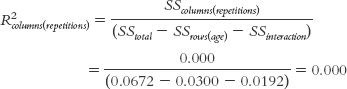
For the second main effect, the one in the columns of the table of cells, the formula is:
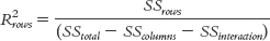
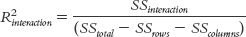
For the interaction, the formula is:
EXAMPLE 14.5
Let’s apply this to the ANOVA we just conducted. We use the statistics in the source table shown in Table 14-19 to calculate R2 for each main effect and the interaction. Here are the calculations for the main effect for age:
Here are the calculations for the main effect for repetitions:
Here are the calculations for the interaction:
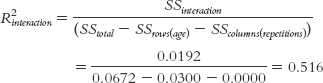
The conventions are the same as those presented in Chapter 12, shown again here in Table 14-20. From this table, we can see that the R2 of 0.63 for the main effect of age and 0.52 for the interaction are very large. The R2 of 0.00 for the main effect of repetitions indicates that there is no observable effect in this study.
| Effect Size | Convention |
|---|---|
| Small | 0.01 |
| Medium | 0.06 |
| Large | 0.14 |
376
Next Steps
Variations on ANOVA
A mixed-
We’ve already seen the flexibility that ANOVA offers in terms of both independent variables and research design. Yet ANOVA is even more flexible than we’ve seen so far in this and the previous two chapters. We described within-
A multivariate analysis of variance (MANOVA) is a form of ANOVA in which there is more than one dependent variable.
Analysis of covariance (ANCOVA) is a type of ANOVA in which a covariate is included so that statistical findings reflect effects after a scale variable has been statistically removed.
A covariate is a scale variable that we suspect associates, or covaries, with the independent variable of interest.
A multivariate analysis of covariance (MANCOVA) is an ANOVA with multiple dependent variables and a covariate.
- A mixed-
design ANOVA is used to analyze the data from a study with at least two independent variables; at least one variable must be within-groups and at least one variable must be between- . In other words, a mixed design includes both a between-groups groups variable and a within- groups variable. - A multivariate analysis of variance (MANOVA) is a form of ANOVA in which there is more than one dependent variable. The word multivariate refers to the number of dependent variables, not the number of independent variables. (Remember, a plain old ANOVA already can handle multiple independent variables.)
- Analysis of covariance (ANCOVA) is a type of ANOVA in which a covariate is included so that statistical findings reflect effects after a scale variable has been statistically removed. Specifically, a covariate is a scale variable that we suspect associates, or covaries, with the independent variable of interest. So ANCOVA statistically subtracts the effect of a possible confounding variable.
- We can also combine the features of a MANOVA and an ANCOVA. A multivariate analysis of covariance (MANCOVA) is an ANOVA with multiple dependent variables and a covariate. MANOVAs, ANCOVAs, and MANCOVAs can each have a between-
groups design, a within- groups design, or even a mixed design. Table 14- 21 shows variations on ANOVA.
| Independent Variables | Dependent Variables | Covariate | |
|---|---|---|---|
| ANOVA | Any number | Only one | None |
| MANOVA | Any number | More than one | None |
| ANCOVA | Any number | Only one | At least one |
| MANCOVA | Any number | More than one | At least one |
377
Let’s consider an example of a mixed-
However, these researchers also included a third independent variable in their analyses. They included not only final exam grades but also grades from the earlier midterm exam. So they had another independent variable, exam, with two levels: midterm and final. Because every student took both exams, this third independent variable is within-
Let’s consider an example of a MANCOVA, an analysis that includes both (a) multiple dependent variables and (b) at least one covariate.
(a) We sometimes use a multivariate analysis when we have several similar dependent variables. Aside from the use of multiple dependent variables, multivariate analyses are not all that different from those with one dependent variable. Essentially, the calculations treat the group of dependent variables as one dependent variable. Although we can follow up a MANOVA by considering the different univariate (single dependent variable) ANOVAs embedded in the MANOVA, we often are most interested in the effect of the independent variables on the composite of dependent variables.
(b) There are often situations in which we suspect that a third variable might be affecting the dependent variable. In these cases, we might conduct an ANCOVA or MANCOVA. We might, for example, have level of education as one of the independent variables and worry that age, which is likely related to level of education, is actually what is influencing the dependent variable, not education. In this case, we could include age as a covariate.
The inclusion of a covariate means that the analysis will look at the effects of the independent variables on the dependent variables after statistically removing the effect of one or more third variables. At its most basic, conducting an ANCOVA is almost like conducting an ANOVA at each level of the covariate. If age were the covariate with level of education as the independent variable and income as the dependent variable, then we’d essentially be looking at a regular ANOVA for each age. We want to answer the question: Given a certain age, does education predict income? Of course, this is a simplified explanation, but that’s the logic behind the procedure. If the calculations find that education has an effect on income among 33-
Researchers conducted a MANCOVA to analyze the results of a study examining military service and marital status within the context of men’s satisfaction within their romantic relationships (McLeland & Sutton, 2005). The independent variables were military service (military, nonmilitary) and marital status (married, unmarried). There were two dependent variables, both measures of relationship satisfaction: the Kansas Marital Satisfaction Scale (KMSS) and the ENRICH Marital Satisfaction Scale (EMS). The researchers also included the covariate of age.
378
Initial analyses also found that age was significantly associated with relationship satisfaction: Older men tended to be more satisfied than younger men. The researchers wanted to be certain that it was military status and marital status, not age, that affected relationship satisfaction, so they controlled for age as a covariate. The MANCOVA led to only one statistically significant finding: Military men were less satisfied than nonmilitary men with respect to their relationships, when controlling for the age of the men. That is, given a certain age, military men of that age are likely to be less satisfied with their relationships than are nonmilitary men of that age.
CHECK YOUR LEARNING
Reviewing the Concepts
- The six steps of hypothesis testing for a two-
way between- groups ANOVA are similar to those for a one- way between- groups ANOVA. - Because we have the possibility of two main effects and an interaction, each step is broken down into three parts, with three sets of hypotheses, comparison distributions, critical F values, F statistics, and conclusions.
- An expanded source table helps us to keep track of the calculations.
- Significant F statistics require post hoc tests to determine where differences lie when there are more than two groups.
- We calculate a measure of effect size, R2, for each main effect and for the interaction.
- Factorial ANOVAs can have a mixed design in addition to a between-
groups design or within- groups design. In a mixed design, at least one of the independent variables is between- groups and at least one of the independent variables is within- groups. - Researchers can also include multiple dependent variables, not just multiple independent variables, in a single study, analyzed with a MANOVA.
- Researchers can add a covariate to an ANOVA and conduct an ANCOVA, which allows us to control for the effect of a variable that is related to the independent variable.
- Researchers can include multiple dependent variables and one or more covariates in an analysis called a MANCOVA.
Clarifying the Concepts
- 14-
9 What is the basic difference between the six steps of hypothesis testing for a two-way between- groups ANOVA and a one- way between- groups ANOVA? - 14-
10 What are the four sources of variability in a two-way ANOVA?
Calculating the Statistics
- 14-
11 Compute the three between-groups degrees of freedom (both main effects and the interaction), the within- groups degrees of freedom, and the total degrees of freedom for the following data:
IV 1, level A; IV 2, level A: 2, 1, 1, 3
IV 1, level B; IV 2, level A: 5, 4, 3, 4
IV 1, level A; IV 2, level B: 2, 3, 3, 3
IV 1, level B; IV 2, level B: 3, 2, 2, 3
- 14-
12 Using the degrees of freedom you calculated in Check Your Learning 14-11, determine critical values, or cutoffs, using a p level of 0.05, for the F statistics of the two main effects and the interaction.
379
Applying the Concepts
- 14-
13 Researchers studied the effect of e-mail messages on students’ final exam grades (Forsyth & Kerr, 1999; Forsyth et al., 2007). To test for possible interactions, participants included students whose first exam grade was either (1) a C, or (2) a D or an F. Participants were randomly assigned to receive several e- mails in one of three conditions: e- mails intended to bolster their self- esteem, e- mails intended to enhance their sense of control over their grades, and e- mails that just included review questions (control group). The accompanying table shows the cell means for the final exam grades (note that some of these are approximate, but all represent actual findings). For simplicity, assume there were 84 participants in the study evenly divided among cells. Self- Esteem (SE) Take Responsibility (TR) Control Group (CG) C 67.31 69.83 71.12 D/F 47.83 60.98 62.13 - From step 1 of hypothesis testing, list the populations for this study.
- Conduct step 2 of hypothesis testing.
- Conduct step 3 of hypothesis testing.
- Conduct step 4 of hypothesis testing.
- The F statistics are 20.84 for the main effect of the independent variable of initial grade, 1.69 for the main effect of the independent variable of type of e-
mail, and 3.02 for the interaction. Conduct step 6 of hypothesis testing.
Solutions to these Check Your Learning questions can be found in Appendix D.