16.3 Multiple Regression
An orthogonal variable is an independent variable that makes a separate and distinct contribution in the prediction of a dependent variable, as compared with the contributions of another variable.
In regression analysis, we explain more of the variability in the dependent variable if we can discover genuine predictors that are separate and distinct. This involves orthogonal variables, independent variables that make separate and distinct contributions in the prediction of a dependent variable, as compared with the contributions of other variables. Orthogonal variables do not overlap each other. For example, the study we discussed earlier explored whether the amount of Facebook use predicted social capital. It is likely that a person’s personality also predicts social capital; for example, we would expect extroverted, or outgoing, people to be more likely to have this kind of social capital than introverted, or shy, people. It would be useful to separate the effects of the amount of Facebook use and extroversion on social capital.
The statistical technique we consider next is a way of quantifying (1) whether multiple pieces of evidence really are better than one, and (2) precisely how much better each additional piece of evidence actually is.
Understanding the Equation
Multiple regression is a statistical technique that includes two or more predictor variables in a prediction equation.
Just as a regression equation using one independent variable is a better predictor than the mean, a regression equation using more than one independent variable is likely to be an even better predictor. This makes sense in the same way that knowing a baseball player’s historical batting average plus knowing that the player continues to suffer from a serious injury is likely to improve our ability to predict the player’s future performance. So it is not surprising that multiple regression is far more common than simple linear regression. Multiple regression is a statistical technique that includes two or more predictor variables in a prediction equation.
Let’s examine an equation that might be used to predict a final exam grade from two variables, number of absences and score on the mathematics portion of the SAT. Table 16-8 repeats the data from Table 16-1, with the added variable of SAT score. (Note that although the scores on number of absences and final exam grade are real-
| Student | Absences | SAT | Exam Grade |
|---|---|---|---|
| 1 | 4 | 620 | 82 |
| 2 | 2 | 750 | 98 |
| 3 | 2 | 500 | 76 |
| 4 | 3 | 520 | 68 |
| 5 | 1 | 540 | 84 |
| 6 | 0 | 690 | 99 |
| 7 | 4 | 590 | 67 |
| 8 | 8 | 490 | 58 |
| 9 | 7 | 450 | 50 |
| 10 | 3 | 560 | 78 |
MASTERING THE CONCEPT
16.5: Multiple regression predicts scores on a single dependent variable from scores on more than one independent variable. Because behavior tends to be influenced by many factors, multiple regression allows us to better predict a given outcome.
441
The computer gives us the printout seen in Figure 16-7. The column in which we’re interested is the one labeled “B,” under “Unstandardized Coefficients.” The first number, across from “(Constant),” is the intercept. The intercept is called constant because it does not change; it is not multiplied by any value of an independent variable. The intercept here is 33.422. The second number is the slope for the independent variable, number of absences. Number of absences is negatively correlated with final exam grade, so the slope, −3.340, is negative. The third number in this column is the slope for the independent variable of SAT score. As we might guess, SAT score and final exam grade are positively correlated; a student with a high SAT score tends to have a higher final exam grade. So the slope, 0.094, is positive. We can put these numbers into a regression equation, with X1 representing the first variable, SAT score, and X2 representing the second variable, final exam grade:

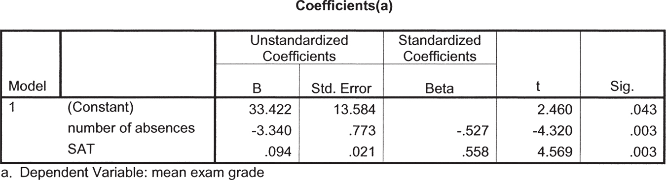
Figure 16-
Once we develop the multiple regression equation, we can input raw scores on number of absences and mathematics SAT score to determine a student’s predicted score on Y. Imagine that our student, Allie, scored 600 on the mathematics portion of the SAT. We already know she planned to miss two classes this semester. What would we predict her final exam grade to be?
442
Based on these two variables, we predict a final exam grade of 83.142 for Allie. How good is this multiple regression equation? From software, we calculated that the proportionate reduction in error for this equation is a whopping 0.93. By using a multiple regression equation with the independent variables of number of absences and SAT score, we have reduced 93% of the error that would result from predicting the mean of 76 for everyone.
When we calculate proportionate reduction in error for a multiple regression, the symbol changes slightly. The symbol is now R2 instead of r2. The capitalization of this statistic is an indication that the proportionate reduction in error is based on more than one independent variable.
Stepwise Multiple Regression and Hierarchical Multiple Regression
Stepwise multiple regression is a type of multiple regression in which a computer program determines the order in which independent variables are included in the equation.
Researchers have several options to choose from when they conduct statistical analyses using multiple regression. One common approach is stepwise multiple regression, a type of multiple regression in which a computer program determines the order in which independent variables are included in the equation. Stepwise multiple regression is used frequently by researchers because it is the default in many computer programs.
When the researcher conducts a stepwise multiple regression, the program implements a series of steps. In the first step, it identifies the independent variable responsible for the most variance in the dependent variable—
If the first independent variable is a statistically significant predictor of the dependent variable, then the program continues to the next step: choosing the second independent variable that, in conjunction with the one already chosen, is responsible for the largest amount of variance in the dependent variable. If the R2 of both independent variables together represents a statistically significant increase over the R2 of just the first independent variable alone, then the program continues to the next step: choosing the independent variable responsible for the next largest amount of variance, and so on. So, at each step, the program assesses whether the change in R2, after adding another independent variable, is statistically significant. If the inclusion of an additional independent variable does not lead to a statistically significant increase in R2 at any step, then the program stops.

443
The strength of using stepwise regression is its reliance on data, rather than theory—
For example, imagine that both depression and anxiety are very strong negative predictors of the quality of one’s romantic relationship. Also imagine that there is a great deal of overlap in the predictive ability of depression and anxiety. That is, once depression is accounted for, anxiety doesn’t add much to the equation; similarly, once anxiety is accounted for, depression doesn’t add much to the equation. It is perhaps the negative affect (or mood) shared by both clusters of symptoms that predicts the quality of one’s relationship.
Now imagine that in one sample, depression turns out to be a slightly better predictor of relationship quality than is anxiety, but just barely. The computer would choose depression as the first independent variable. Because of the overlap between the two independent variables, the addition of anxiety would not be statistically significant. A stepwise regression would pinpoint depression, but not anxiety, as a predictor of relationship quality. That finding would suggest that anxiety is not a good predictor of the quality of your romantic relationship even though it could be extremely important.
Now imagine that in a second sample, anxiety is a slightly better predictor of relationship quality than is depression, but just barely. This time, the computer would choose anxiety as the first independent variable. Now the addition of depression would not be statistically significant. This time, a stepwise regression would pinpoint anxiety, but not depression, as a predictor of relationship quality. So the problem with using stepwise multiple regression is that two samples with very similar data can, and sometimes do, lead to drastically different conclusions.
Hierarchical multiple regression is a type of multiple regression in which the researcher adds independent variables into the equation in an order determined by theory.
That is why another common approach is hierarchical multiple regression, a type of multiple regression in which the researcher adds independent variables into the equation in an order determined by theory. A researcher might want to know the degree to which depression predicts relationship quality but knows that there are other independent variables that also affect relationship quality. Based on a reading of the literature, that researcher might decide to enter other independent variables into the equation before adding depression.
For example, the researcher might add age, a measure of social skills, and the number of years the relationship has lasted. After adding these independent variables, the researcher would add depression. If the addition of depression leads to a statistically significant increase in R2, then the researcher has evidence that depression predicts relationship quality over and above those other independent variables. As with stepwise multiple regression, we’re interested in how much each additional independent variable adds to the overall variance explained. We look at the increase in R2 with the inclusion of each new independent variable or variables and we predetermine the order (or hierarchy) in which variables are entered into a hierarchical regression equation.
MASTERING THE CONCEPT
16.6: In multiple regression, we determine whether each added independent variable increases the amount of variance in the dependent variable that we can explain. In stepwise multiple regression, the computer program determines the order in which independent variables are added, whereas in hierarchical multiple regression, the researcher chooses the order. In both cases, however, we report the increase in R2 with the inclusion of each new independent variable or variables.
444
The strength of hierarchical multiple regression is that it is grounded in theory that we can test. In addition, we’re less likely to identify a statistically significant predictor just by chance (a Type I error) because a well-
Multiple Regression in Everyday Life
With the development of increasingly more powerful computers and the availability of ever-
Bing Travel is an attempt at an end run, using mathematical prediction tools, to help savvy airline consumers either beat or wait out the airlines’ price hikes. In 2007, Bing Travel’s precursor, Farecast.com, claimed a 74.5% accuracy rate for its predictions. Zillow.com does for real estate what Bing Travel does for airline tickets. Using archival land records, Zillow.com predicts U.S. housing prices and claims to be accurate to within 10% of the actual selling price of a given home.
Another company, Inrix, predicts the dependent variable, traffic, using the independent variables of the weather, traveling speeds of vehicles that have been outfitted with Global Positioning Systems (GPS), and information about events such as rock concerts. It even suggests, via cell phone or in-
Next Steps
Structural Equation Modeling (SEM)
Structural equation modeling (SEM) is a statistical technique that quantifies how well sample data “fit” a theoretical model that hypothesizes a set of relations among multiple variables.
A statistical (or theoretical) model is a hypothesized network of relations, often portrayed graphically, among multiple variables.
We’re going to introduce an approach to data analysis that is infinitely more flexible and visually more expressive than multiple regression. Structural equation modeling (SEM) is a statistical technique that quantifies how well sample data “fit” a theoretical model that hypothesizes a set of relations among multiple variables. Here, we are discussing “fit” in much the same way you might try on some new clothes and say, “That’s a good fit” or “That really doesn’t fit!” Statisticians who use SEM refer to the “model” that they are testing. In this case, a statistical (or theoretical) model is a hypothesized network of relations, often portrayed graphically, among multiple variables.
Instead of thinking of variables as “independent” variables or “dependent” variables, SEM encourages researchers to think of variables as a series of connections. Consider an independent variable such as the number of hours spent studying. What predicts how many hours a person will study? We answer that by thinking of hours studying as a dependent variable with its own set of independent variables. An independent variable in one study can become a dependent variable in another study. SEM quantifies a network of relations, so some of the variables are independent variables that predict other variables later in the network, as well as dependent variables that are predicted by other variables earlier in the network. This is why we will refer to variables without the usual adjectives of independent or dependent as we discuss SEM.
445
Path is the term that statisticians use to describe the connection between two variables in a statistical model.
Path analysis is a statistical method that examines a hypothesized model, usually by conducting a series of regression analyses that quantify the paths between variables at each succeeding step in the model.
Language Alert! In the historical development of SEM, the analyses based on this kind of diagram were called path analyses for the fairly obvious reason that the arrows represented “paths”—factors that lead to whatever the next variable in the model happened to be. Path is the term that statisticians use to describe the connection between two variables in a statistical model. Path analysis is a statistical method that examines a hypothesized model, usually by conducting a series of regression analyses that quantify the paths at each succeeding step in the model.
Path analysis is used rarely these days because the more powerful technique of SEM can better quantify the relations among variables in a model. But we still find the term path to be a more intuitive way to describe the flow of behavior through a network of variables, and the word path continues to be used in structural equation models. SEM uses a statistic much like the correlation coefficient to indicate the relation between any two variables. Like a path through a forest, a path could be small and barely discernible (close to 0) or large and easy to follow (closer to −1.00 or 1.00).
Manifest variables are the variables in a study that we can observe and that are measured.
Latent variables are the ideas that we want to research but cannot directly measure.
In SEM, we start with measurements called manifest variables, the variables in a study that we can observe and that are measured. We assess something that we can observe in an attempt to understand the underlying main idea in which we’re interested. In SEM, these main idea variables are called latent variables, the ideas that we want to research but cannot directly measure. For example, we cannot actually see the latent variable we call “shyness,” but we still try to measure shyness in the manifest variables using self-
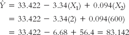
Let’s examine one published SEM study. In a longitudinal study, researchers examined whether receiving good parenting at age 17 predicted emotional adjustment at age 26 (Dumas, Lawford, Tieu, & Pratt, 2009). They explored the relations among four latent variables in a sample of 100 adolescents in Ontario, Canada. The latent variables were the following:
- Positive parenting, an estimate of whether an adolescent received good parenting as assessed by three self-
report manifest variables at age 17 - Story ending (a variable called narrative coherent positive resolution by the researchers), an estimate based on stories that participants were asked to tell at age 26 about their most difficult life experience and that included the manifest variables of the positivity of the story’s ending, the negativity of the story’s ending, whether the ending was coherent, and whether the story had a resolution
- Identity maturity with respect to religion, politics, and career at age 26, quantified via the manifest variables of achievement (strong identity in these areas), moratorium (still deciding with respect to these areas), and diffusion (weak identity in these areas)
- Emotional adjustment, assessed at age 26 by the manifest variables of optimism, depression, and general well-
being
Note that higher scores on all four latent variables indicate a more positive outcome. Figure 16-8 depicts the researchers’ model.
Figure 16-
To understand the story of this model, we need to understand only three components—
446
The squares above or below each circle represent the measurement tools used to operationalize each latent variable. These are the manifest variables, the ones that can be observed. Let’s look at “Story ending,” the latent variable related to the stories that the 26-
Once we understand the latent variables (as measured by the three or more manifest variables), all that’s left for us to understand is the arrows that represent each path. The numbers on each path give us a sense of the relation between each pair of variables. Similar to correlation coefficients, the sign of the number indicates the direction of the relation, either negative or positive, and the value of the number indicates the strength of the relation. Although this is a simplification, these basic rules will allow you to “read” the story in the diagram of the model.
So how does this SEM diagram address the research question about the effects of good parenting? We’ll start on the left and read across. Notice the two paths that lead from positive parenting to story ending and to identity maturity. The numbers are 0.31 and 0.41, respectively. These are fairly large positive numbers. They suggest that receiving positive parenting at age 17 leads to a healthier interpretation of a negative life experience and to a well-
Now notice the two-
447
When you encounter a model such as SEM, follow these basic steps: First, figure out what variables the researcher is studying. Then, look at the numbers to see which variables are related and look at the signs of the numbers to see the direction of the relation.
CHECK YOUR LEARNING
Reviewing the Concepts
- Multiple regression is used to predict a dependent variable from more than one independent variable. Ideally, these variables are distinct from one another in such a way that they contribute uniquely to the predictions.
- We can develop a multiple regression equation and input specific scores for each independent variable to determine the predicted score on the dependent variable.
- Multiple regression is the backbone of many online tools that we can use for predicting everyday variables such as traffic or home prices.
- In stepwise multiple regression, a computer program determines the order in which independent variables are tested; in hierarchical multiple regression, the researcher determines the order.
- Structural equation modeling (SEM) allows us to examine the “fit” of a sample’s data to a hypothesized model of the relations among multiple variables, the latent variables that we hypothesize to exist but cannot see.
Clarifying the Concepts
- 16-
10 What is multiple regression, and what are its benefits over simple linear regression?
Calculating the Statistics
- 16-
11 Write the equation for the line of prediction using the following output from a multiple regression analysis: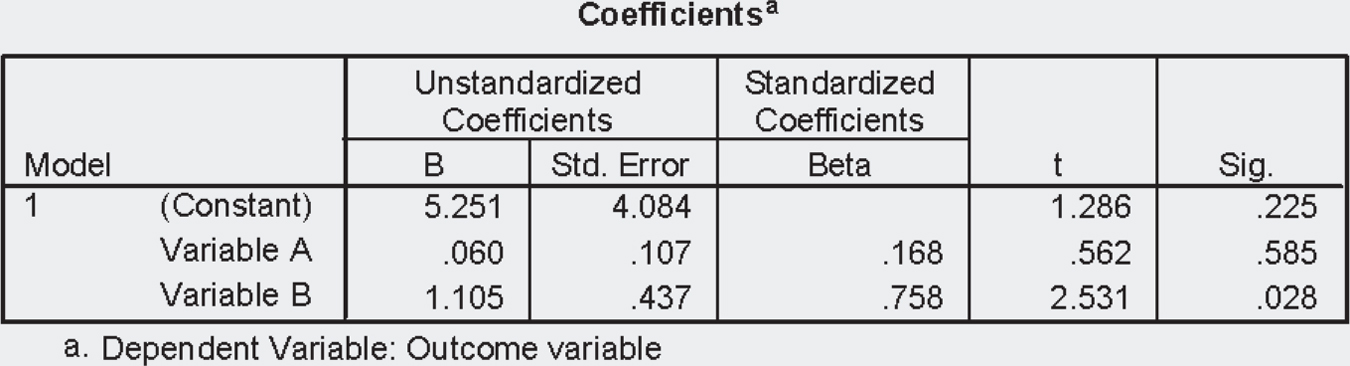
- 16-
12 Use the equation for the line you created in Check Your Learning 16-11 to make predictions for each of the following: - X1 = 40, X2 = 14
- X1 = 101, X2 = 39
- X1 = 76, X2 = 20
Applying the Concepts
- 16-
13 The accompanying computer printout shows a regression equation that predicts GPA from three independent variables: hours slept per night, hours studied per week, and admiration for Pamela Anderson, the B-level actress whom many view as tacky. The data are from some of our statistics classes. (Note: Hypothesis testing shows that all three independent variables are statistically significant predictors of GPA!) 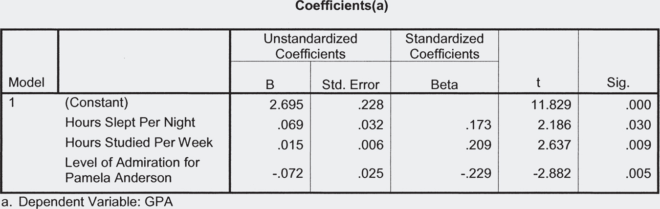
- Based on these data, what is the regression equation?
- If someone reports that he typically sleeps 6 hours a night, studies 20 hours per week, and has a Pamela Anderson admiration level of 4 (on a scale of 1–
7, with 7 indicating the highest level of admiration), what would you predict for his GPA? - What does the negative sign in the slope for the independent variable, level of admiration for Pamela Anderson, tell you about this variable’s predictive association with GPA?
Solutions to these Check Your Learning questions can be found in Appendix D.