Chapter 16 Exercises
Clarifying the Concepts
Question 16.1
What does regression add above and beyond what we learn from correlation?
Question 16.2
How does the regression line relate to the correlation of the two variables?
Question 16.3
Is there any difference between 
and a predicted score for Y?
Question 16.4
What do each of the symbols stand for in the formula for the regression equation: 
Question 16.5
The equation for a line is
= a + b(X). Define the symbols a and b.
Question 16.6
What are the three steps to calculate the intercept?
Question 16.7
When is the intercept not meaningful or useful?
Question 16.8
What does the slope tell us?
Question 16.9
Why do we also call the regression line the line of best fit?
Question 16.10
How are the sign of the correlation coefficient and the sign of the slope related?
Question 16.11
What is the difference between a small standard error of the estimate and a large one?
Question 16.12
Why are explanations of the causes behind relations explored with regression limited in the same way they are with correlation?
Question 16.13
What is the connection between regression to the mean and the bell-
Question 16.14
Explain why the regression equation is a better source of predictions than is the mean.
Question 16.15
What is the SStotal?
Question 16.16
When drawing error lines between data points and the regression line, why is it important that these lines be perfectly vertical?
Question 16.17
What are the basic steps to calculate the proportionate reduction in error?
Question 16.18
What information does the proportionate reduction in error give us?
Question 16.19
What is an orthogonal variable?
Question 16.20
If you know the correlation coefficient, how can you determine the proportionate reduction in error?
Question 16.21
Why is multiple regression often more useful than simple linear regression?
452
Question 16.22
What is the difference between stepwise multiple regression and hierarchical multiple regression?
Question 16.23
What is the primary weakness of stepwise multiple regression?
Question 16.24
How does structural equation modeling (SEM) differ from multiple regression?
Question 16.25
What is the difference between a latent variable and a manifest variable?
Question 16.26
What are the three primary components that we need to understand an SEM diagram? Explain what each component means.
Calculating the Statistics
Question 16.27
Using the following information, make a prediction for Y, given an X score of 2.9:
Variable X: M = 1.9, SD = 0.6
Variable Y: M = 10, SD = 3.2
Pearson correlation of variables X and Y = 0.31
Transform the raw score for the independent variable to a z score.
Calculate the predicted z score for the dependent variable.
Transform the z score for the dependent variable back into a raw score.
Question 16.28
Using the following information, make a prediction for Y, given an X score of 8:
Variable X: M = 12, SD = 3
Variable Y: M = 74, SD = 18
Pearson correlation of variables X and Y = 0.46
Transform the raw score for the independent variable to a z score.
Calculate the predicted z score for the dependent variable.
Transform the z score for the dependent variable back into a raw score.
Calculate the y intercept, a.
Calculate the slope, b.
Write the equation for the line.
Draw the line on an empty scatterplot, basing the line on predicted Y values for X values of 0, 1, and 18.
Question 16.29
Let’s assume we know that age is related to bone density, with a Pearson correlation coefficient of −0.19. (Notice that the correlation is negative, indicating that bone density tends to be lower at older ages than at younger ages.) Assume we also know the following descriptive statistics:
Age of people studied: 55 years on average, with a standard deviation of 12 years
Bone density of people studied: 1000 mg/cm2 on average, with a standard deviation of 95 mg/cm2
Virginia is 76 years old. What would you predict her bone density to be? To answer this question, complete the following steps:
Transform the raw score for the independent variable to a z score.
Calculate the predicted z score for the dependent variable.
Transform the z score for the dependent variable back into a raw score.
Calculate the y intercept, a.
Calculate the slope, b.
Write the equation for the line.
Draw the line on an empty scatterplot, basing the line on predicted Y values for X values of 0, 1, and 18.
Question 16.30
Given the regression line
= −6 + 0.41(X), make predictions for each of the following:
X = 25
X = 50
X = 75
Question 16.31
Given the regression line
= 49 − 0.18(X), make predictions for each of the following:
X = −31
X = 65
X = 14
Question 16.32
Data are provided here with descriptive statistics, a correlation coefficient, and a regression equation: r = 0.426,
= 219.974 + 186.595(X).
| X | Y |
|---|---|
| 0.13 | 200.00 |
| 0.27 | 98.00 |
| 0.49 | 543.00 |
| 0.57 | 385.00 |
| 0.84 | 420.00 |
| 1.12 | 312.00 |
| MX = 0.57 | MY = 326.333 |
| SDX = 0.333 | SDY = 145.752 |
Using this information, compute the following estimates of prediction error:
Calculate the sum of squared error for the mean, SStotal.
Now, using the regression equation provided, calculate the sum of squared error for the regression equation, SSerror.
Using your work, calculate the proportionate reduction in error for these data.
Check that this calculation of r2 equals the square of the correlation coefficient.
Compute the standardized regression coefficient.
Question 16.33
Data are provided here with descriptive statistics, a correlation coefficient, and a regression equation: r = 0.52,
= 2.643 + 0.469(X).
| X | Y |
|---|---|
| 4.00 | 6.00 |
| 6.00 | 3.00 |
| 7.00 | 7.00 |
| 8.00 | 5.00 |
| 9.00 | 4.00 |
| 10.00 | 12.00 |
| 12.00 | 9.00 |
| 14.00 | 8.00 |
| MX = 8.75 | MY = 6.75 |
| SDX = 3.031 | SDY = 2.727 |
Using this information, compute the following estimates of prediction error:
Calculate the sum of squared error for the mean, SStotal.
Now, using the regression equation provided, calculate the sum of squared error for the regression equation, SSerror.
Using your work, calculate the proportionate reduction in error for these data.
Check that this calculation of r2 equals the square of the correlation coefficient.
Compute the standardized regression coefficient.
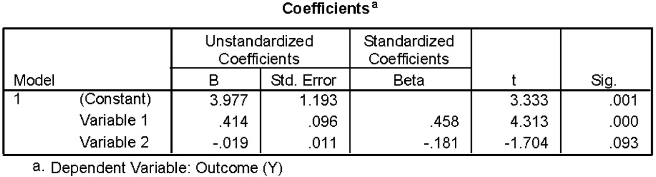
Question 16.34
Use this output from a multiple regression analysis to answer the following questions:
Write the equation for the line of prediction.
Use the equation for part (a) to make predictions for: Variable 1 = 6, variable 2 = 60
Use the equation for part (a) to make predictions for: Variable 1 = 9, variable 2 = 54.3
Use the equation for part (a) to make predictions for: Variable 1 = 13, variable 2 = 44.8
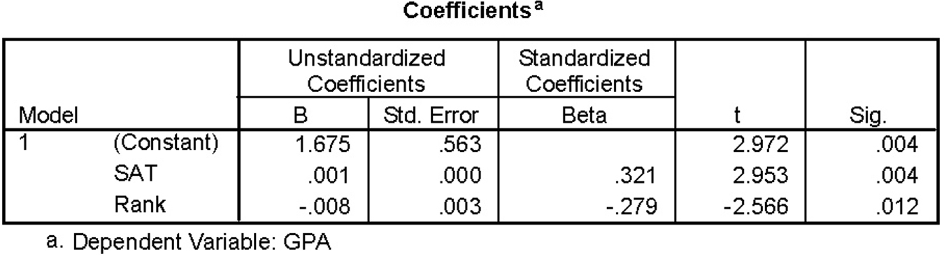
Question 16.35
Use this output from a multiple regression analysis to answer the following questions:
Write the equation for the line of prediction.
Use the equation for part (a) to make predictions for: SAT = 1030, rank = 41
Use the equation for part (a) to make predictions for: SAT = 860, rank = 22
Use the equation for part (a) to make predictions for: SAT = 1060, rank = 8
Question 16.36
Assume that a researcher is interested in variables that might affect infant birth weight. The researcher performs a stepwise multiple regression to predict birth weight and includes the following independent variables: (1) how many miles the mother lives from a grocery store, (2) number of cigarettes the mother smokes per day, (3) weight of the mother. If the statistical program produces a regression that includes only the first two independent variables, what can we conclude about the third variable, weight of mother?
Question 16.37
Refer to the structural equation model (SEM) depicted in Figure 16-8 to answer the following:
Which two variables are most strongly related to each other?
Is positive parenting at age 17 directly related to emotional adjustment at age 26? How do you know?
Is positive parenting at age 17 directly related to identity maturity at age 26? How do you know?
What is the difference between the variables represented in boxes and those represented in circles?
Applying the Concepts
Question 16.38
Weight, blood pressure, and regression: Several studies have found a correlation between weight and blood pressure.
454
Explain what is meant by a correlation between these two variables.
If you were to examine these two variables with simple linear regression instead of correlation, how would you frame the question? (Hint: The research question for correlation would be: Is weight related to blood pressure?)
What is the difference between simple linear regression and multiple regression?
If you were to conduct a multiple regression instead of a simple linear regression, what other independent variables might you include?
Question 16.39
Temperature, hot chocolate sales, and prediction: Running a football stadium involves innumerable predictions. For example, when stocking up on food and beverages for sale at the game, it helps to have an idea of how much will be sold. In the football stadiums in colder climates, stadium managers use expected outdoor temperature to predict sales of hot chocolate.
What is the independent variable in this example?
What is the dependent variable?
As the value of the independent variable increases, what can we predict would happen to the value of the dependent variable?
What other variables might predict this dependent variable? Name at least three.
Question 16.40
Age, hours studied, and prediction: In How It Works 15.2, we calculated the correlation coefficient between students’ age and number of hours they study per week. The correlation between these two variables is 0.49.
Elif’s z score for age is −0.82. What would we predict for the z score for the number of hours she studies per week?
John’s z score for age is 1.2. What would we predict for the z score for the number of hours he studies per week?
Eugene’s z score for age is 0. What would we predict for the z score for the number of hours he studies per week?
For part (c) explain why the concept of regression to the mean is not relevant (and why you didn’t really need the formula).
Question 16.41
Consideration of Future Consequences scale, z scores, and raw scores: A study of Consideration of Future Consequences (CFC) found a mean score of 3.51, with a standard deviation of 0.61, for the 664 students in the sample (Petrocelli, 2003).
Imagine that your z score on the CFC score was −1.2. What would your raw score be? Use symbolic notation and the formula. Explain why this answer makes sense.
Imagine that your z score on the CFC score was 0.66. What would your raw score be? Use symbolic notation and the formula. Explain why this answer makes sense.
Question 16.42
The GRE, z scores, and raw scores: The verbal subtest of the Graduate Record Examination (GRE) has a population mean of 500 and a population standard deviation of 100 by design (the quantitative subtest has the same mean and standard deviation).
Convert the following z scores to raw scores without using a formula: (i) 1.5, (ii) −0.5, (iii) −2.0
Now convert the same z scores to raw scores using symbolic notation and the formula: (i) 1.5, (ii) −0.5, (iii) −2.0
Question 16.43
Hours studied, grade, and regression: A regression analysis of data from some of our statistics classes yielded the following regression equation for the independent variable (hours studied) and the dependent variable (grade point average [GPA]):
= 2.96 + 0.02(X).
If you plan to study 8 hours per week, what would you predict your GPA will be?
If you plan to study 10 hours per week, what would you predict your GPA will be?
If you plan to study 11 hours per week, what would you predict your GPA will be?
Create a graph and draw the regression line based on these three pairs of scores.
Do some algebra, and determine the number of hours you’d have to study to have a predicted GPA of the maximum possible, 4.0. Why is it misleading to make predictions for anyone who plans to study this many hours (or more)?
Question 16.44
Precipitation, violence, and limitations of regression: Does the level of precipitation predict violence? Dubner and Levitt (2006b) reported on various studies that found links between rain and violence. They mentioned one study by Miguel, Satyanath, and Sergenti that found that decreased rain was linked with an increased likelihood of civil war across a number of African countries they examined. Referring to the study’s authors, Dubner and Levitt state, “The causal effect of a drought, they argue, was frighteningly strong.”
What is the independent variable in this study?
What is the dependent variable?
What possible third variables might play a role in this connection? That is, is it just the lack of rain that’s causing violence, or is it something else? (Hint: Consider the likely economic base of many African countries.)
Question 16.45
Cola consumption, bone mineral density, and limitations of regression: Does one’s cola consumption predict one’s bone mineral density? Using regression analyses, nutrition researchers found that older women who drank more cola (but not more of other carbonated drinks) tended to have lower bone mineral density, a risk factor for osteoporosis (Tucker, Morita, Qiao, Hannan, Cupples, & Kiel, 2006). Cola intake, therefore, does seem to predict bone mineral density.
455
Explain why we cannot conclude that cola intake causes a decrease in bone mineral density.
The researchers included a number of possible third variables in their regression analyses. Among the included variables were physical activity score, smoking, alcohol use, and calcium intake. They included the possible third variables first, and then added the bone density measure. Why would they have used multiple regression in this case? Explain.
How might physical activity play a role as a third variable? Discuss its possible relation to both bone density and cola consumption.
How might calcium intake play a role as a third variable? Discuss its possible relation to both bone density and cola consumption.
Question 16.46
Tutoring, mathematics performance, and problems with regression: A researcher conducted a study in which children with problems lear ning mathematics were offered the opportunity to purchase time with special tutors. The number of weeks that children met with their tutors varied from 1 to 20. He found that the number of weeks of tutoring predicted these children’s mathematics performance and recommended that parents of such children send them for tutoring.
List one problem with that interpretation. Explain your answer.
If you were to develop a study that uses a multiple regression equation instead of a simple linear regression equation, what additional variables might be good independent variables? List at least one variable that can be manipulated (e.g., weeks of tutoring) and at least one variable that cannot be manipulated (e.g., parents’ years of education).
How would you develop the multiple regression equation using stepwise multiple regression? (Note: There is more than one specific answer. In your response, demonstrate that you understand the basic process of stepwise multiple regression.)
How would you develop the multiple regression equation using hierarchical multiple regression? (Note: There is more than one specific answer. In your response, demonstrate that you understand the basic process of hierarchical multiple regression.)
Describe a situation in which stepwise multiple regression might be preferred.
Describe a situation in which hierarchical multiple regression might be preferred.
Question 16.47
Anxiety, depression, and simple linear regression: We analyzed data from a larger data set that one of the authors used for previous research (Nolan, Flynn, & Garber, 2003). In the current analyses, we used regression to look at factors that predict anxiety over a 3-
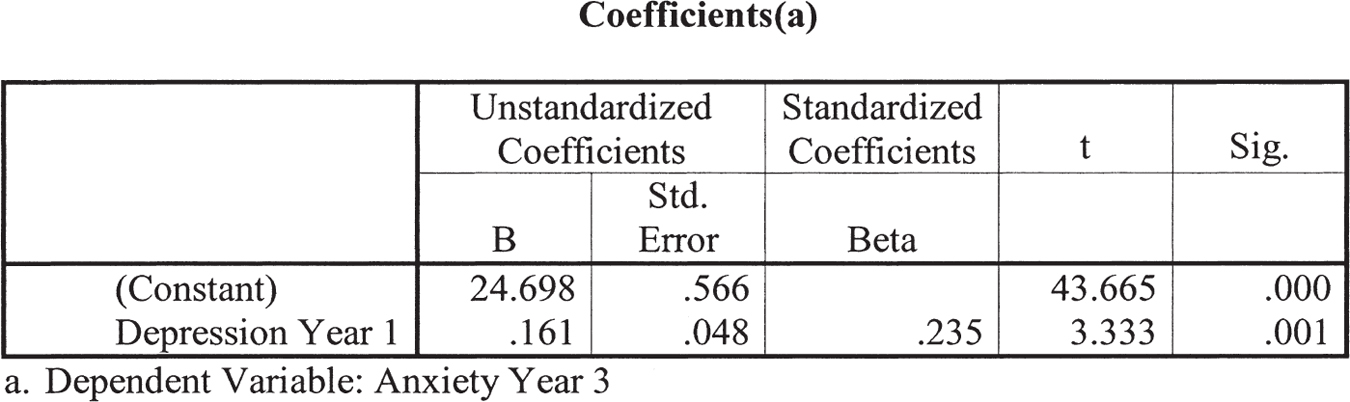
From this software output, write the regression equation.
As depression at year 1 increases by 1 point, what happens to the predicted anxiety level for year 3? Be specific.
If someone has a depression score of 10 at year 1, what would we predict for her anxiety score at year 3?
If someone has a depression score of 2 at year 1, what would we predict for his anxiety score at year 3?
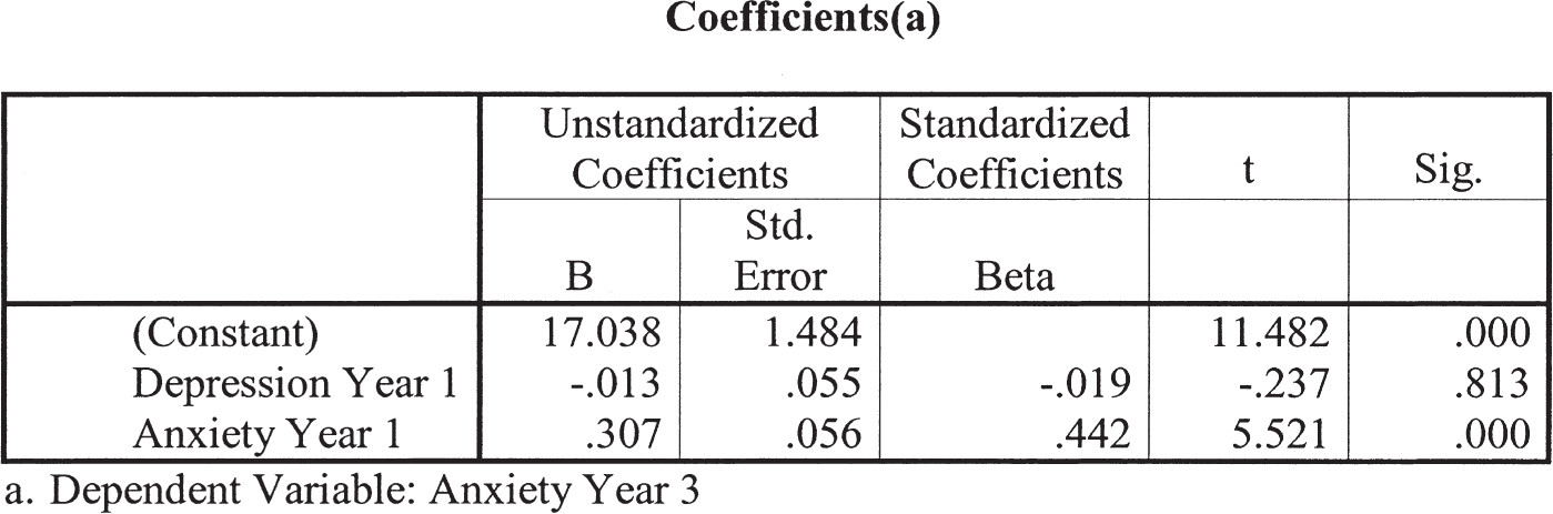
Question 16.48
Anxiety, depression, and multiple regression: We conducted a second regression analysis on the data from Exercise 16.47. In addition to depression at year 1, we included a second independent variable to predict anxiety at year 3. We also included anxiety at year 1. (We might expect that the best predictor of anxiety at a later point in time is one’s anxiety at an earlier point in time.) Here is the output for that analysis.
456
From this software output, write the regression equation.
As the first independent variable, depression at year 1, increases by 1 point, what happens to the predicted score on anxiety at year 3?
As the second independent variable, anxiety at year 1, increases by 1 point, what happens to the predicted score on anxiety at year 3?
Compare the predictive utility of depression at year 1 using the regression equation in Exercise 16.47 and using the regression equation you just wrote in 16.48(a). In which regression equation is depression at year 1 a better predictor? Given that we’re using the same sample, is depression at year 1 actually better at predicting anxiety at year 3 in one regression equation versus the other? Why do you think there’s a difference?
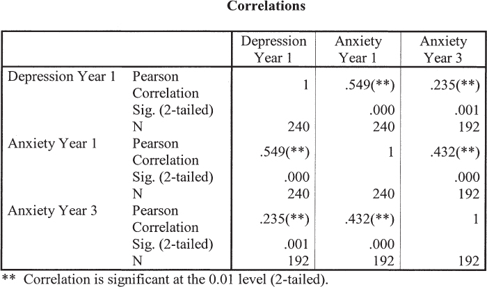
The accompanying table is the correlation matrix for the three variables. As you can see, all three are highly correlated with one another. If we look at the intersection of each pair of variables, the number next to “Pearson correlation” is the correlation coefficient. For example, the correlation between “Anxiety year 1” and “Depression year 1” is .549. Which two variables show the strongest correlation? How might this explain the fact that depression at year 1 seems to be a better predictor when it’s the only independent variable than when anxiety at year 1 also is included? What does this tell us about the importance of including third variables in the regression analyses when possible?
Let’s say you want to add a fourth independent variable. You have to choose among three possible independent variables: (1) a variable highly correlated with both independent variables and the dependent variable, (2) a variable highly correlated with the dependent variable but not correlated with either independent variable, and (3) a variable not correlated with either of the independent variables or with the dependent variable. Which of the three variables is likely to make the multiple regression equation better? That is, which is likely to increase the proportionate reduction in error? Explain.
Question 16.49
Cohabitation, divorce, and prediction: A study by the Institute for Fiscal Studies (Goodman & Greaves, 2010) found that parents’ marital status when a child was born predicted the likelihood of the relationship’s demise. Parents who were cohabitating when their child was born had a 27% chance of breaking up by the time the child was 5, whereas those who were married when their child was born had a 9% chance of breaking up by the time the child was 5—
What are the independent and dependent variables used in this study?
Were the researchers likely to have used simple linear regression or multiple regression for their analyses? Explain your answer.
In your own words, explain why the ability of marital status at the time of a child’s birth to predict divorce within 5 years almost disappeared when other variables were considered. Explain your answer.
Name at least one additional “third variable” that might have been at play in this situation. Explain your answer.
Question 16.50
Google, the flu, and third variables: The New York Times reported: “Several years ago, Google, aware of how many of us were sneezing and coughing, created a fancy equation on its Web site to figure out just how many people had influenza. The math works like this: people’s location + flurelated search queries on Google + some really smart algorithms = the number of people with the flu in the United States” (Bilton, 2013; http:/
A friend who knows you’re taking statistics asks you to explain what this means in statistical terms. In your own words, what is it likely that the Google statisticians did?
The problem was that their “fancy equation” didn’t work. It estimated that 11% of the U.S. population had the flu, but the real number was only 6%. The New York Times article warned against taking data out of context. What do you think may have gone wrong in this case? (Hint: Think about your own Google searches and the varied reasons you have for conducting those searches.)
Question 16.51
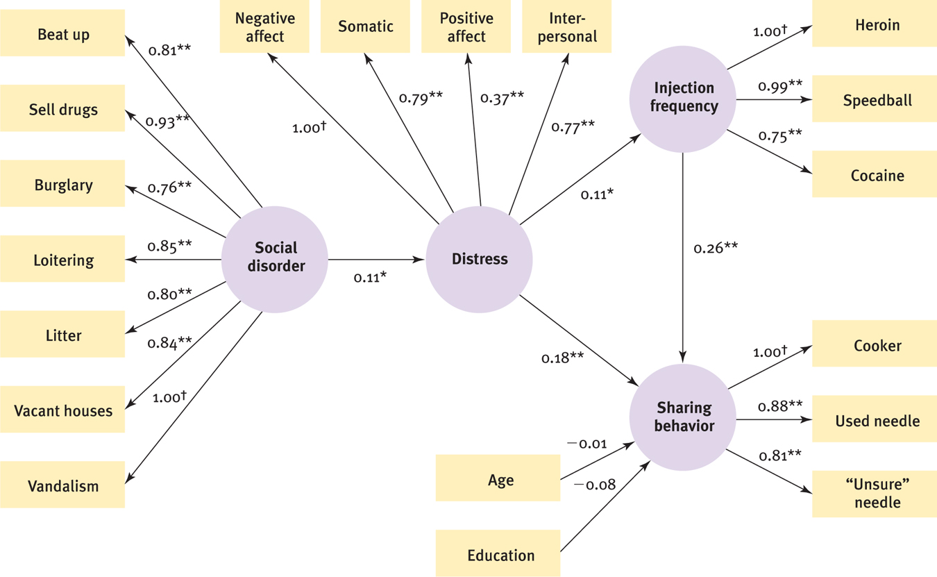
Neighborhood social disorder and structural equation modeling: The attached figure is from a journal article entitled “Neighborhood Social Disorder as a Determinant of Drug Injection Behaviors: A Structural Equation Modeling Approach” (Latkin, Williams, Wang, & Curry, 2005).
What are the four latent variables examined in this study?
What manifest variables were used to operationalize social disorder? Based on these manifest variables, explain in your own words what you think the authors mean by “social disorder.”
Looking only at the latent variables, which two variables seem to be most strongly related to each other? What is the number on that path? Is it positive or negative, and what does the sign of the number indicate about the relation between these variables?
Looking only at the latent variables, what overall story is this model telling? (Note: Asterisks indicate relations that inferential statistics indicate are likely “real,” even if they are fairly small.)
Question 16.52
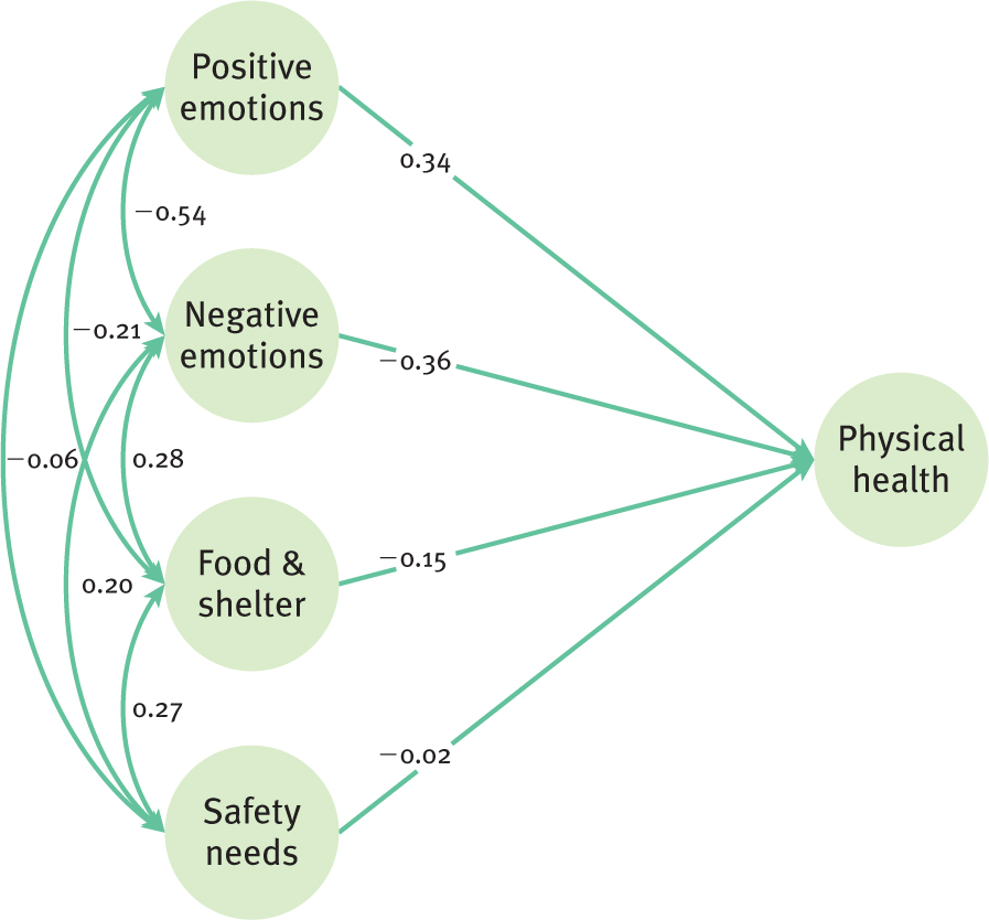
Physical health around the world and structural equation modeling: The figure on the next page shows the latent variables of a structural equation model (Pressman, Gallagher, & Lopez, 2013). Researchers examined predictors of mental health in more than 150,000 people from 142 countries. Use the figure to answer the following questions.
Explain the relations of positive and negative emotions to physical health.
In the explanation of their structural equation model, the researchers stated about positive emotions and negative emotions: “Together, they accounted for almost half (46.1%) of the variance in health” (p. 1). From your understanding of variance, explain what the researchers mean by this statement.
A reporter in the Huffington Post wrote about this research: “Is the concept of emotions having an effect on health a “First World” problem? According to a new study, no, it is not—
and in fact, the association may be even stronger in developing nations” (http:/ /www.huffingtonpost.com/ , 2013). What is the reporter implying by this statement in terms of causality?2013/ 03/ 25/ positivity-and-good-health-lower-income-countries-emotions_n_2916288.html Knowing only about the relations you described in part (a), list several third variables that might be responsible for the relation between emotions and physical health.
Food and shelter along with safety needs are included in the model. How does this make the relations you described in part (a) more convincing as explanations.
Question 16.53
Sugar, diabetes, and multiple regression: New York Times reporter Mark Bittman wrote: “A study published in the journal PLoS One links increased consumption of sugar with increased rates of diabetes by examining the data on sugar availability and the rate of diabetes in 175 countries over the past decade. And after accounting for many other factors, the researchers found that increased sugar in a population’s food supply was linked to higher diabetes rates independent of rates of obesity” (2013; http:/
Explain how the researchers may have used multiple regression to analyze these data.
Why did Bittman emphasize that the researchers accounted for many other factors?
List at least three other factors that the researchers may have included.
Bittman also wrote: “In other words, according to this study, obesity doesn’t cause diabetes: sugar does. The study demonstrates this with the same level of confidence that linked cigarettes and lung cancer in the 1960s.” Explain in your own words why Bittman likely feels justified in drawing a causal conclusion from correlational research.
Putting It All Together
Question 16.54
Corporate political contributions, profits, and regression: Researchers studied whether corporate political contributions predicted profits (Cooper, Gulen, & Ovtchinnikov, 2007). From archival data, they determined how many political candidates each company supported with financial contributions, as well as each company’s profit in terms of a percentage. The accompanying table shows data for five companies. (Note: The data points are hypothetical but are based on averages for companies falling in the 2nd, 4th, 6th, and 8th deciles in terms of candidates supported. A decile is a range of 10%, so the 2nd decile includes those with percentiles between 10 and 19.9.)
| Number of Candidates Supported | Profit (%) |
|---|---|
| 6 | 12.37 |
| 17 | 12.91 |
| 39 | 12.59 |
| 62 | 13.43 |
| 98 | 13.42 |
Create the scatterplot for these scores.
Calculate the mean and standard deviation for the variable “number of candidates supported.”
Calculate the mean and standard deviation for the variable “profit.”
Calculate the correlation between number of candidates supported and profit.
Calculate the regression equation for the prediction of profit from number of candidates supported.
Create a graph and draw the regression line.
What do these data suggest about the political process?
What third variables might be at play here?
Compute the standardized regression coefficient.
How does this coefficient relate to other information you know?
Draw a conclusion about your analysis based on what you know about hypothesis testing with simple linear regression.
Question 16.55
Age, hours studied, and regression: In How It Works 15.2, we calculated the correlation coefficient between students’ age and number of hours they study per week. The mean for age is 21, and the standard deviation is 1.789. The mean for hours studied is 14.2, and the standard deviation is 5.582. The correlation between these two variables is 0.49. Use the z score formula.
João is 24 years old. How many hours would we predict he studies per week?
Kimberly is 19 years old. How many hours would we predict she studies per week?
Seung is 45 years old. Why might it not be a good idea to predict how many hours per week he studies?
From a mathematical perspective, why is the word regression used? (Hint: Look at parts (a) and (b), and discuss the scores on the first variable with respect to their mean versus the predicted scores on the second variable with respect to their mean.)
Calculate the regression equation.
Use the regression equation to predict the number of hours studied for a 17-
year- old student and for a 22- year- old student. Using the four pairs of scores that you have (age and predicted hours studied from part (b), and the predicted scores for a score of 0 and 1 from calculating the regression equation), create a graph that includes the regression line.
Why is it misleading to include young ages such as 0 and 5 on the graph?
Construct a graph that includes both the scatterplot for these data and the regression line. Draw vertical lines to connect each dot on the scatterplot with the regression line.
Construct a second graph that includes both the scatterplot and a line for the mean for hours studied, 14.2. The line will be horizontal and will begin at 14.2 on the y-axis. Draw vertical lines to connect each dot on the scatterplot with the regression line.
Part (i) is a depiction of the error we make if we use the regression equation to predict hours studied. Part (j) is a depiction of the error we make if we use the mean to predict hours studied (i.e., if we predict that everyone has the mean of 16.2 on hours studied per week). Which one appears to have less error? Briefly explain why the error is less in one situation.
Calculate the proportionate reduction in error the long way.
Explain what the proportionate reduction in error that you calculated in part (l) tells us. Be specific about what it tells us about predicting using the regression equation versus predicting using the mean.
Demonstrate how the proportionate reduction in error could be calculated using the shortcut. Why does this make sense? That is, why does the correlation coefficient give us a sense of how useful the regression equation will be?
Compute the standardized regression coefficient.
How does this coefficient relate to other information you know?
Draw a conclusion about your analysis based on what you know about hypothesis testing with regression.