17.4 Cramer’s V, the Effect Size for Chi Square
Cramer’s V is the standard effect size used with the chi-
MASTERING THE FORMULA
 17-
17- The numerator is the chi-
A hypothesis test tells us only that there is a likely effect—
Cramer’s V is the standard effect size used with the chi-

χ2 is the test statistic we just calculated, N is the total number of participants in the study (the lower-
EXAMPLE 17.3
For the clown example, we calculated a chi-

Now that we have the effect size, we must ask what it means. As with other effect sizes, Jacob Cohen (1992) has developed guidelines, shown in Table 17-9, for determining whether a particular effect is small, medium, or large. The guidelines vary based on the size of the contingency table. When the smaller of the two degrees of freedom for the row and column is 1, we use the guidelines in the second column. When the smaller of the two degrees of freedom is 2, we use the guidelines in the third column. And when it is 3, we use the guidelines in the fourth column. As with the other guidelines for judging effect sizes, such as those for Cohen’s d, the guidelines are not cutoffs. Rather, they are rough indicators to help researchers gauge a finding’s importance.
The effect size for the clowning and pregnancy study was 0.18. The smaller of the two degrees of freedom, that for the row and that for the column, was 1 (in fact, both were 1). So we use the second column in Table 17-9. This Cramer’s V falls about halfway between the effect-
χ2 (1, N = 186) = 6.08, p < 0.05, Cramer’s V 5 0.18
| Effect size | When dfrow/column = 1 | When dfrow/column = 2 | When dfrow/column = 3 |
|---|---|---|---|
| Small | 0.10 | 0.07 | 0.06 |
| Medium | 0.30 | 0.21 | 0.17 |
| Large | 0.50 | 0.35 | 0.29 |
477
Graphing Chi-Square Percentages
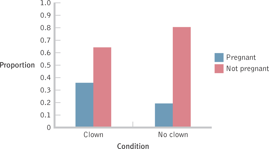
In addition to calculating Cramer’s V, we can graph the data. A visual depiction of the pattern of results is an effective way to understand the size of the relation between two variables assessed using the chi-
EXAMPLE 17.4
For the women entertained by a clown, we calculate the proportion who became pregnant and the proportion who did not. For the women not entertained by a clown, we again calculate the proportion who became pregnant and the proportion who did not. The calculations for the proportions are below.
In each case, we’re dividing the number of a given outcome by the total number of women in that group. The proportions are called conditional proportions because we’re not calculating the proportions out of all women in the study; we’re calculating proportions for women in a certain condition. We calculate the proportion of women who became pregnant, for example, conditional on their having been entertained by a clown.
Entertained by a clown
- Became pregnant: 33/93 = 0.355
- Did not become pregnant: 60/93 = 0.645
Not entertained by a clown
- Became pregnant: 18/93 = 0.194
- Did not become pregnant: 75/93 = 0.806
We can put those proportions into a table (such as Table 17-10). For each category of entertainment (clown, no clown), the proportions should add up to 1.00; or if we used percentages, they should add up to 100%.
| Conditional Proportions | |||
|---|---|---|---|
| Pregnant | Not pregnant | ||
| Clown | 0.355 | 0.645 | 1.00 |
| No clown | 0.194 | 0.806 | 1.00 |
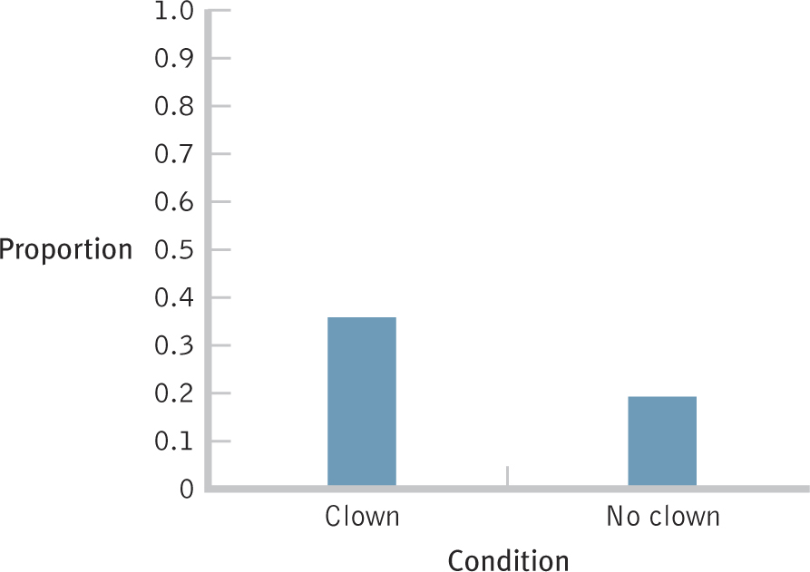
We can now graph the conditional proportions, as in Figure 17-5. Alternately, we could have simply graphed the two rates at which women got pregnant—

Figure 17-

Figure 17-
478
Relative Risk
Public health statisticians like John Snow (Chapter 1) are called epidemiologists. They often think about the size of an effect with chi square in terms of relative risk, a measure created by making a ratio of two conditional proportions. It is also called relative likelihood or relative chance. As with Figure 17-5, we calculate the chance of getting pregnant with clown entertainment after IVF by dividing the number of pregnancies in this group by the total number of women entertained by clowns:
Relative risk is a measure created by making a ratio of two conditional proportions; also called relative likelihood or relative chance.
33/93 = 0.355
479
We then calculate the chance of getting pregnant with no clown entertainment after IVF by dividing the number of pregnancies in this group by the total number of women not entertained by clowns:
18/93 = 0.194
If we divide the chance of getting pregnant having been entertained by clowns by the chance of getting pregnant not having been entertained by clowns, then we get the relative likelihood:
0.355/0.194 = 1.830
Based on the relative risk calculation, the chance of getting pregnant when IVF is followed by clown entertainment is 1.83 times the chance of getting pregnant when IVF is not followed by clown entertainment. This matches the impression that we get from the graph.
Alternately, we can reverse the ratio, dividing the chance of becoming pregnant without clown entertainment, 0.194, by the chance of becoming pregnant following clown entertainment, 0.355. This is the relative likelihood for the reversed ratio:

0.194/0.355 = 0.546
MASTERING THE CONCEPT
17.3: We can quantify the size of an effect with chi square through relative risk, also called relative likelihood. By making a ratio of two conditional proportions, we can say, for example, that one group is twice as likely to show some outcome or, conversely, that the other group is one-
This number gives us the same information in a different way. The chance of getting pregnant when IVF is followed by no entertainment is 0.55 (or about half) the chance of getting pregnant when IVF is followed by clown entertainment. Again, this matches the graph; one bar is about half that of the other.
(Note: When this calculation is made with respect to diseases, it is referred to as relative risk [rather than relative likelihood].) We should be careful when relative risks and relative likelihoods are reported, however. We must always be aware of base rates. If, for example, a certain disease occurs in just 0.01% of the population (that is, 1 in 10,000) and is twice as likely to occur among people who eat ice cream, then the rate is 0.02% (2 in 10,000) among those who eat ice cream. Relative risks and relative likelihoods can be used to scare the general public unnecessarily—
480
Next Steps
Adjusted Standardized Residuals
Chi-
Adjusted standardized residual is the difference between the observed frequency and the expected frequency for a cell in a chi-
A cell’s residual is the difference between the expected frequency and the observed frequency for that cell, but we take it a step further. We calculate an adjusted standardized residual, the difference between the observed frequency and the expected frequency for a cell in a chi-
Does this sound familiar? The adjusted standardized frequency is kind of like a z statistic for each cell (Agresti & Franklin, 2006). A larger adjusted standardized residual indicates that an observed frequency is farther from its expected frequency than a smaller adjusted standardized residual indicates. And as with a z statistic, we’re not concerned with the sign. A large positive adjusted standardized residual and a large negative adjusted standardized residual tell us the same thing. If it’s large enough, then we’re willing to conclude that the observed frequency really is different from what we would expect if the null hypothesis were true.
Also like a z statistic, any time a cell has an adjusted standardized residual that is at least 2 (whether the sign is positive or negative), we are willing to conclude that the cell’s observed frequency is different from its expected frequency. Some statisticians prefer a more stringent criterion, drawing this conclusion only if an adjusted standardized residual is larger than 3 (again, whether the sign is positive or negative). Regardless of the criterion used, the method and logic for determining the probabilities of z statistics and determining adjusted standardized residuals are the same.
Adjusted standardized residuals are too complicated to calculate without the aid of a computer, but we’ll show you a software printout of the adjusted standardized residuals for the clown therapy study. Figure 17-7 shows the printout from the SPSS software package. The row labeled “Count” includes the observed frequencies. The “Expected Count” row includes the expected frequencies. The “Adjusted Residual” row includes the adjusted standardized residuals. So, for example, the upper-

Figure 17-
481
CHECK YOUR LEARNING
Reviewing the Concepts
- After completing a hypothesis test, it is wise to calculate an effect size as well. The appropriate effect-
size measure for the chi- square test for independence is Cramer’s V. - We can depict the effect size visually by calculating and graphing conditional proportions so that we can compare the rates of a certain outcome in each of two or more groups.
- Another way to consider the size of an effect is through relative risk, a ratio of conditional proportions for each of two groups.
- A statistically significant chi-
square hypothesis test does not tell us exactly which cells are farther from their expected frequencies than would occur if the two variables were independent. We must calculate adjusted standardized residuals to identify these cells.
Clarifying the Concepts
- 17-
9 What is the effect-size measure for chi- square tests and how is it calculated?
Calculating the Statistics
- 17-
10 Assume you are interested in whether students with different majors tend to have different political affiliations. You ask U.S. psychology majors and business majors to indicate whether they are Democrats or Republicans. Of 67 psychology majors, 36 indicated that they are Republicans and 31 indicated that they are Democrats. Of 92 business majors, 54 indicated that they are Republicans and 38 indicated that they are Democrats. Calculate the relative likelihood of being a Republican, given that a person is a business major as opposed to a psychology major.
Applying the Concepts
- 17-
11 In Check Your Learning 17-8, you were asked to conduct a chi- square test on a Chicago Police Department study comparing two types of lineups for suspect identification: simultaneous lineups and sequential lineups (Mecklenburg et al., 2006). - Calculate the appropriate measure of effect size for this study.
- Create a graph of the conditional proportions for these data.
- Calculate the relative likelihood of a suspect being accurately identified in the simultaneous lineups versus the sequential lineups.
Solutions to these Check Your Learning questions can be found in Appendix D.
482