18.1 Ordinal Data and Correlation
The statistical tests we discuss in this section allow researchers to draw conclusions from data that do not meet the assumptions for a parametric test, such as when the data are rank ordered. In this section, we learn how to convert scale data to ordinal data. Then we examine four tests that can be used with ordinal data: nonparametric versions of the Pearson correlation coefficient (the Spearman rank-
497
When the Data Are Ordinal

A 2006 University of Chicago News Office press release proclaimed, “Americans and Venezuelans Lead the World in National Pride.” Researchers from the University of Chicago’s National Opinion Research Center (NORC) surveyed citizens of 33 countries (Smith & Kim, 2006) and developed two different kinds of national pride scores: pride in specific accomplishments of their nations, like science or sports (which they called domain-
So, the researchers had two sets of national pride scores—
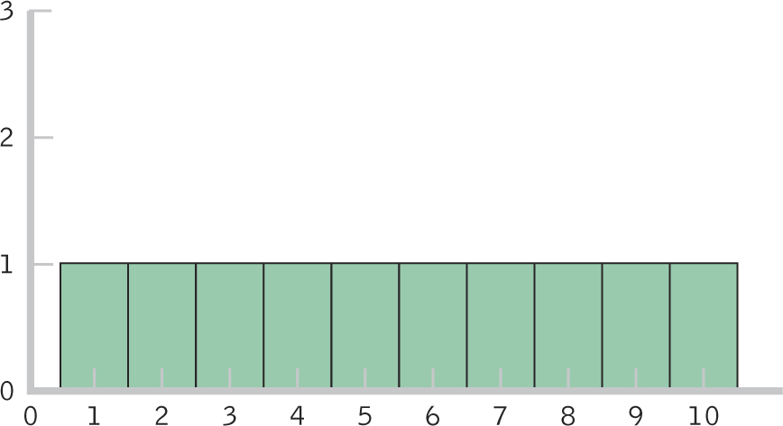
Figure 18-
We wondered about other possible precursors of national pride, such as competitiveness. Because the researchers provided ordinal data, the only way we can explore these interesting hypotheses is by using nonparametric statistics. Parametric statistics are appropriate for scale data, but they are not appropriate for ordinal data. As we noted in Chapter 17, the very nature of an ordinal variable means that it will not meet the assumptions of a scale dependent variable and a normally distributed population. As we can see in Figure 18-1, the shape of a distribution of ordinal variables is rectangular because every participant has a different rank.
Fortunately, the logic of many nonparametric statistics will be familiar to students. This is because many of the nonparametric statistical tests are specific alternatives to parametric statistical tests. These nonparametric tests may be used whenever assumptions for a parametric test are not met. In this chapter, we’ll consider four such tests (shown in Table 18-1): (1) a nonparametric equivalent for the Pearson correlation coefficient, the Spearman rank-
| Design | Parametric Test | Nonparametric Test |
|---|---|---|
| Association between two variables | Pearson correlation coefficient | Spearman rank- |
| Two groups; within- |
Paired- |
Wilcoxon signed- |
| Two groups; between- |
Independent- |
Mann– |
| More than two groups; between- |
One- |
Kruskal– |
498
EXAMPLE 18.1
Nonparametric tests for ordinal data are typically used in one of two situations. First and most obviously, we use nonparametric tests when the sample data are ordinal. Second, we use nonparametric tests when the dependent variable suggests that the underlying population distribution is greatly skewed, a common situation when the sample size is small. This second reason is likely why the national pride researchers converted their data to ranks (Smith & Kim, 2006). Figure 18-2 shows a histogram of their full set of data for the variable accomplishment-
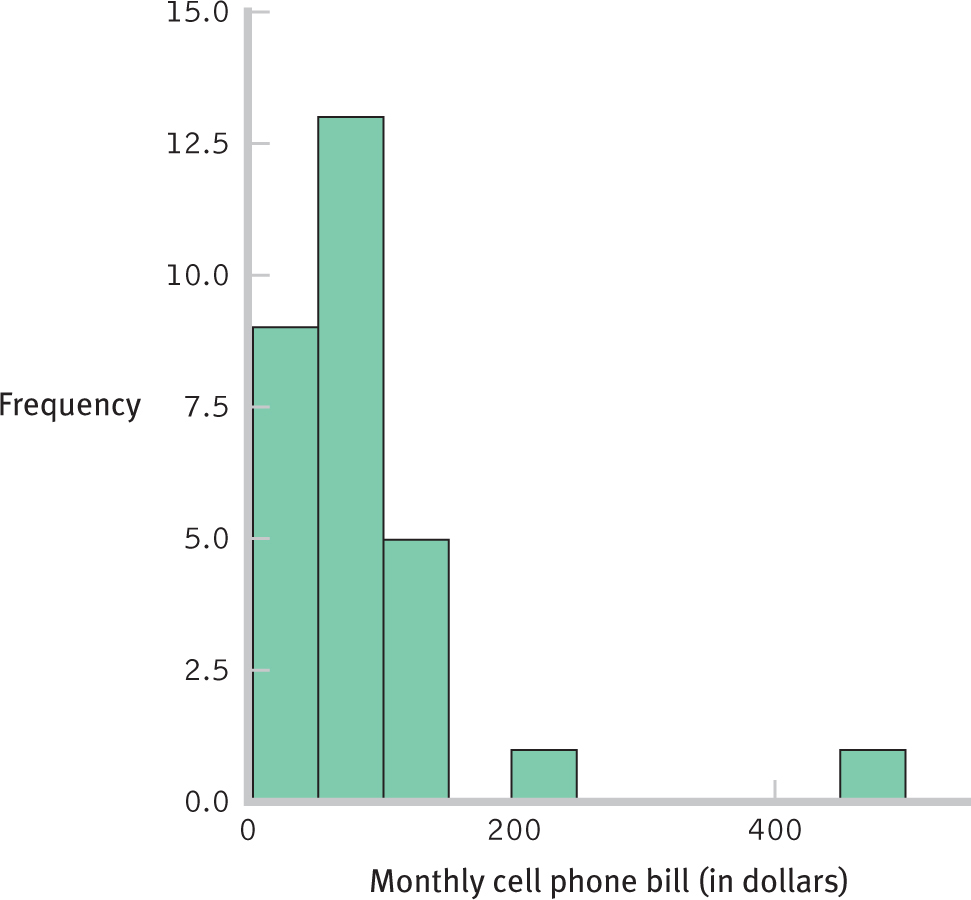
Figure 18-
It is appropriate to transform scale data to ordinal data whenever the data from a small sample are skewed. For example, look what happens to the following five data points for income when we change the data from scale to ordinal. In the first row, the one that includes the scale data, there is a severe outlier ($550,000) and the sample data suggest a skewed distribution. In the second row, the severe outlier merely becomes the last ranking. The ranked data do not have an outlier.
499
- Scale: $24,000 $27,000 $35,000 $46,000 $550,000
- Ordinal: 1 2 3 4 5
In the next section, we’ll transform scale data to ordinal data so that we can calculate the Spearman rank-
The Spearman Rank-Order Correlation Coefficient
The Spearman rank-
Many everyday, automatic decisions are based on rank-
MASTERING THE CONCEPT
18.1: We calculate a Spearman rank-
EXAMPLE 18.2
To see how the Spearman rank-
A correlation between these variables, if found, would be evidence that countries’ levels of accomplishment-
To convert scale data to ordinal data, we simply organize the data from highest to lowest (or lowest to highest, if that makes more sense) and then rank them. Table 18-2 shows the conversion of accomplishment-
| Country | Pride Score | Pride Rank |
|---|---|---|
| United States | 4.0 | 1 |
| South Africa | 2.7 | 2 |
| Austria | 2.4 | 3.5 |
| Canada | 2.4 | 3.5 |
| Chile | 2.3 | 5 |
| Japan | 1.8 | 6 |
| Hungary | 1.6 | 7 |
| France | 1.5 | 8 |
| Norway | 1.3 | 9 |
| Slovenia | 1.1 | 10 |
Now that we have the ranks, we can compute the Spearman correlation coefficient. We first need to include both sets of ranks in the same table, as in the second and third columns in Table 18-3. We then calculate the difference (D) between each pair of ranks, as in the fourth column. The differences always add up to 0, so we must square the differences, as in the last column. As we have frequently done with squared differences in the past, we sum them—
500
∑D2 = (0 + 64 + 2.25 + 0.25 + 0 + 1 + 1 + 4 + 25 + 1) = 98.5
| Country | Pride Rank | Competitiveness Rank |
Difference (D) | Squared Difference (D2) |
|---|---|---|---|---|
| United States | 1 | 1 | 0 | 0 |
| South Africa | 2 | 10 | −8 | 64 |
| Austria | 3.5 | 2 | 1.5 | 2.25 |
| Canada | 3.5 | 3 | 0.5 | 0.25 |
| Chile | 5 | 5 | 0 | 0 |
| Japan | 6 | 7 | −1 | 1 |
| Hungary | 7 | 8 | −1 | 1 |
| France | 8 | 6 | 2 | 4 |
| Norway | 9 | 4 | 5 | 25 |
| Slovenia | 10 | 9 | 1 | 1 |
501
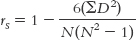
The formula for calculating the Spearman correlation coefficient includes the sum of the squared differences that we just calculated, 98.5. The formula is:
MASTERING THE FORMULA
18-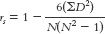 . The numerator includes a constant, 6, as well as the sum of the squared differences between ranks for each participant. The denominator is calculated by multiplying the sample size, N, by the square of the sample size minus 1.
Aside from the sum of squared differences, the only other information we need is the sample size, N, which is 10 in this example. (The number 6 is a constant; it is always included in the calculation of the Spearman correlation coefficient.) The Spearman correlation coefficient, therefore, is:
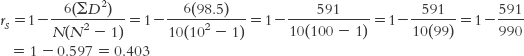
The Spearman correlation coefficient is 0.40.
The interpretation of the Spearman correlation coefficient is identical to that for the Pearson correlation coefficient. The coefficient can range from −1, a perfect negative correlation, to 1, a perfect positive correlation. A correlation coefficient of 0 indicates no relation between the two variables. As with the Pearson correlation coefficient, it is not the sign of the Spearman correlation coefficient that indicates the strength of a relation. So, for example, a coefficient of −0.66 indicates a stronger association than does a coefficient of 0.23. Finally, as with the Pearson correlation coefficient, we can implement the six steps of hypothesis testing to determine whether the Spearman correlation coefficient is statistically significantly different from 0. If we do decide to conduct hypothesis testing, we can find the critical values for the Spearman correlation coefficient in Appendix B.7.
Like the Pearson correlation coefficient, the Spearman correlation coefficient does not tell us about causation. It is possible that there is a causal relation in one of two directions. The relation between competitiveness (variable A) and accomplishment-
CHECK YOUR LEARNING
Reviewing the Concepts
- Nonparametric statistics are used when all variables are nominal, when the dependent variable is ordinal, and when the sample suggests both that the underlying population distribution is skewed and that the sample size is small.
- Nonparametric tests for ordinal data are used when the data are already ordinal or when it is clear that the assumptions are severely violated. In the latter case, the scale data must be converted to ordinal data.
- When we want to calculate a correlation between two ordinal variables, we calculate a Spearman rank-
order correlation coefficient, which is interpreted in the same way as a Pearson correlation coefficient. - As with the Pearson correlation coefficient, the Spearman correlation coefficient does not tell us about causation. It simply quantifies the magnitude and direction of association between two ordinal variables.
502
Clarifying the Concepts
- 18-
1 Describe a common situation in which we use nonparametric tests other than chi-square tests.
Calculating the Statistics
- 18-
2 Convert the following scale data to ordinal or ranked data, starting with a rank of 1 for the smallest data point.Observation Variable 1 Variable 2 1 1.30 54.39 2 1.80 50.11 3 1.20 53.39 4 1.06 44.89 5 1.80 48.50 - 18-
3 Compute the Spearman correlation coefficient for the data listed in Check Your Learning 18-2.
Applying the Concepts
- 18-
4 Here are IQ scores for 10 people: 88, 90, 91, 99, 103, 103, 104, 112, 114, and 139.- Why might it be better to use a nonparametric test than a parametric test in this case?
- Convert the scores for IQ (a scale variable) to ranks (an ordinal variable).
- What happens to the outlier when the scores are converted from a scale measure to an ordinal measure?
Solutions to these Check Your Learning questions can be found in Appendix D.