4.2 Measures of Variability
Variability is a numerical way of describing how much spread there is in a distribution.
People often poked fun at trashy Japanese products after World War II. Sometimes their transistor radios, for example, worked pretty well, but sometimes they didn’t work at all. They just weren’t reliable. However, after Japanese companies started applying Deming’s insight that the definition of high quality was low variability, the tiny nation needed just 3 years to become an industrial powerhouse whose reputation for high-
MASTERING THE CONCEPT
4.3: Variability is the second most common concept (after central tendency) to help us understand the shape of a distribution. Common indicators of variability are range, variance, and standard deviation.
Range
The range is a measure of variability calculated by subtracting the lowest score (the minimum) from the highest score (the maximum).
The range is the easiest measure of variability to calculate. The range is a measure of variability calculated by subtracting the lowest score (the minimum) from the highest score (the maximum). Maximum and minimum are sometimes substituted in this formula to describe the highest and lowest scores, and some statistical computer programs abbreviate these as max and min. The range is represented in a formula as:
87
MASTERING THE FORMULA
4-
range = Xhighest − Xlowest
Here are the scores for countries’ numbers of top finishes in the World Cup that we discussed earlier in the chapter. As before, we’ll omit countries with a score of 0 top finishes.
1 1 1 1 2 2 2 2 2 2 3 3 4 6 8 10
EXAMPLE 4.8
We can determine the highest and lowest scores either by reading through the data or, more easily, by glancing at the frequency table for these data.
STEP 1: Determine the highest score.
In this case, the highest score is 10.
STEP 2: Determine the lowest score.
In this case, the lowest score is 1.
STEP 3: Calculate the range by subtracting the lowest score from the highest score:
range = Xhighest − Xlowest = 10 − 1 = 9
The range can be a useful first indicator of variability, but it is influenced only by the highest and lowest scores. All the other scores in between could be clustered near the highest score, huddled near the center, spread out evenly, or have some other unexpected pattern. We can’t know based only on the range.
Variance
Variance is the average of the squared deviations from the mean.
Variance is the average of the squared deviations from the mean. When something varies, it must vary from (or be different from) some standard. That standard is the mean. So when we compute variance, that number describes how far a distribution varies around the mean. A small number indicates a small amount of spread or deviation around the mean, and a larger number indicates a great deal of spread or deviation around the mean. Post–
EXAMPLE 4.9
A deviation from the mean is the amount that a score in a sample differs from the mean of the sample; also called a deviation.
Students who seek therapy at university counseling centers often do not attend many sessions. For example, in one study, the median number of therapy sessions was 3 and the mean was 4.6 (Hatchett, 2003). Let’s examine the spread of fictional scores for a sample of five students: 1, 2, 4, 4, and 10 therapy sessions, with a mean of 4.2. We find out how far each score deviates from the mean by subtracting the mean from every score. First, we label the column that lists the scores with an X. Here, the second column includes the results we get when we subtract the mean from each score, or X − M. We call each of these a deviation from the mean (or just a deviation)—the amount that a score in a sample differs from the mean of the sample.
88
| X | X − M |
|---|---|
| 1 | −3.2 |
| 2 | −2.2 |
| 4 | −0.2 |
| 4 | −0.2 |
| 10 | 5.8 |
But we can’t just take the mean of the deviations. If we do (and if you try this, don’t forget the signs—
When we ask students for ways to eliminate the negative signs, two suggestions typically come up: (1) Take the absolute value of the deviations, thus making them all positive, or (2) square all the scores, again making them all positive. It turns out that the latter, squaring all the deviations, is how statisticians solve this problem. Once we square the deviations, we can take their average and get a measure of variability. Later (using a beautifully descriptive term created by our students), we will “unsquare” those deviations in order to calculate the standard deviation.
To recap:
STEP 1: Subtract the mean from every score.
We call these deviations from the mean.
STEP 2: Square every deviation from the mean.
We call these squared deviations.
STEP 3: Sum all of the squared deviations.
This is often called the sum of squared deviations, or the sum of squares, for short.
STEP 4: Divide the sum of squares by the total number in the sample (N).
This number represents the mathematical definition of variance—
The sum of squares, symbolized as SS, is the sum of each score’s squared deviation from the mean.
To calculate the variance for the therapy session data, we add a third column to contain the squares of each of the deviations. Then we add all of these numbers up to compute the sum of squares (symbolized as SS), the sum of each score’s squared deviation from the mean. In this case, the sum of the squared deviations is 48.80, so the average squared deviation is 48.80/5 = 9.76. Thus, the variance equals 9.76.
| X | X − M | (X − M)2 |
|---|---|---|
| 1 | −3.20 | 10.24 |
| 2 | −2.20 | 4.84 |
| 4 | −0.20 | 0.04 |
| 4 | −0.20 | 0.04 |
| 10 | 5.80 | 33.64 |
89
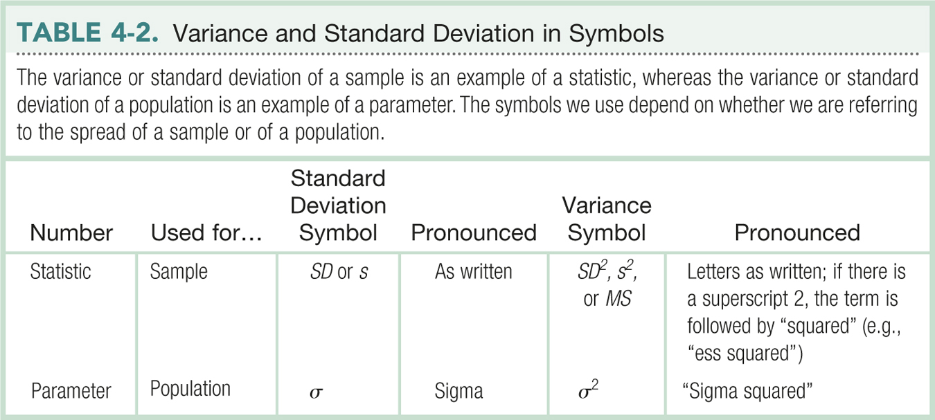
Language Alert! We need a few more symbols to use symbolic notation to represent the idea of variance. Each of these symbols represents the same idea (variance) applied to slightly different situations. The symbols that represent the variance of a sample include SD2, s2, and MS. The first two symbols, SD2 and s2, both represent the words standard deviation squared. The symbolic notation MS comes from the words mean square (referring to the average of the squared deviations). We’ll use SD2 at this point, but we will alert you when we switch to other symbols for variance later. The variance of the sample uses all three symbolic notations; however, the variance of a population uses just one symbol: σ2 (pronounced “sigma squared”). Table 4-2 summarizes the symbols and language used to describe different versions of the mean and variance, but we will keep reminding you as we go along.
We already know all the other symbols needed to calculate variance: X to indicate the individual scores, M to indicate the mean, and N to indicate the sample size.
MASTERING THE FORMULA
4-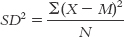 . To calculate variance, subtract the mean (M) from every score (X) to calculate deviations from the mean; then square these deviations, sum them, and divide by the sample size (N). By summing the squared deviations and dividing by sample size, we are taking their mean.
As you can see, variance is really just a mean—
Standard Deviation
EXAMPLE 4.10
The standard deviation is the square root of the average of the squared deviations from the mean; it is the typical amount that each score varies, or deviates, from the mean.
Language Alert! Variance and standard deviation refer to the same core idea. The standard deviation is more useful because it is the typical amount that each score varies from the mean. Mathematically, the standard deviation is the square root of the average of the squared deviations from the mean, or, more simply, the square root of the variance. The beauty of the standard deviation—
For example, the numbers of therapy sessions for the five students were 1, 2, 4, 4, and 10, with a mean of 4.2. The typical score does not vary from the mean by 9.76. The variance is based on squared deviations, not deviations, so it is too large. When we ask our students how to solve this problem, they invariably say, “Unsquare it,” and that’s just what we do. We take the square root of variance to come up with a much more useful number, the standard deviation. The square root of 9.76 is 3.12. Now we have a number that “makes sense” to us. We can now say that the typical number of therapy sessions for students in this sample is 4.2 and the typical amount a student varies from that is 3.12.
90
As you read journal articles, you often will see the mean and standard deviation reported as: (M = 4.2, SD = 3.12). A glance at the original data (1, 2, 4, 4, 10) tells us that these numbers make sense: 4.2 does seem to be approximately in the center, and scores do seem to vary from 4.2 by roughly 3.12. The score of 10 is a bit of an outlier—
MASTERING THE FORMULA
4- . We simply take the square root of the variance.
We didn’t actually need a formula to get the standard deviation. We just took the square root of the variance. Perhaps you guessed the symbols for standard deviation by just taking the square root of those for variance. With a sample, standard deviation is either SD or s. With a population, standard deviation is σ. Table 4-2 presents this information concisely. We can write the formula showing how standard deviation is calculated from variance:
We can also write the formula showing how standard deviation is calculated from the original X’s, M, and N:
MASTERING THE FORMULA
4-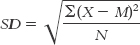 . To determine standard deviation, subtract the mean from every score to calculate deviations from the mean. Then, square the deviations from the mean. Sum the squared deviations, then divide by the sample size. Finally, take the square root of the mean of the squared deviations.
Next Steps
The interquartile range is a measure of the distance between the first and third quartiles.
The first quartile marks the 25th percentile of a data set.
The third quartile marks the 75th percentile of a data set.
The Interquartile Range
As we noted earlier in the chapter, the range has a major limitation: it is completely dependent on the maximum and minimum scores. For example, the $17 million home at the high end or the shack at the low end of the distribution skew a distribution of home prices. Whenever we have outliers, the range will be an exaggerated measure of the variability. Fortunately, we have an alternative to the range: the interquartile range.
The interquartile range is a measure of the distance between the first and third quartiles. As we learned earlier, the median marks the 50th percentile of a data set. Similarly, the first quartile marks the 25th percentile of a data set, and the third quartile marks the 75th percentile of a data set. Essentially, the first and third quartiles are the medians of the two halves of the data—
MASTERING THE FORMULA
4-
Here are the steps for finding the interquartile range:
Step 1: Calculate the median.
Step 2: Look at all of the scores below the median. The median of these scores, the lower half of the scores, is the first quartile, often called Q1 for short.
Step 3: Look at all of the scores above the median. The median of these scores, the upper half of the scores, is the third quartile, often called Q3 for short.
Step 4: Subtract Q1 from Q3. The interquartile range, often abbreviated as IQR, is the difference between the first and third quartiles: IQR = Q3 − Q1.
91
Because the interquartile range is the distance between the 25th and 75th percentile of the data, it can be thought of as the range of the middle 50% of the data.
The interquartile range has an important advantage over the range. Because it is not based on the minimum and maximum—
MASTERING THE CONCEPT
4.4: The interquartile range is the distance from the 25th percentile (first quartile) to the 75th percentile (third quartile). It is often a better measure of variability than the range because it is not affected by outliers.
EXAMPLE 4.11
Here are countries’ top finishes in the World Cup that we examined earlier in the chapter; as we did before, we omitted countries with a score of 0.
1 1 1 1 2 2 2 2 2 2 3 3 4 6 8 10
Earlier we calculated the median of these scores as the mean of the 8th and 9th scores, 2. We now take the first 8 scores: 1, 1, 1, 1, 2, 2, 2, 2. If we divide the number of scores, 8, by 2 and add 1/2, we get 4.5. The median of these scores—
We’ll do the same with the top half of the scores: 2, 2, 3, 3, 4, 6, 8, 10. Again, there are 8 scores, so the median of these scores—
Along with the minimum, median, and maximum, the first and third quartiles provide us with an overview of the data. These five numbers—
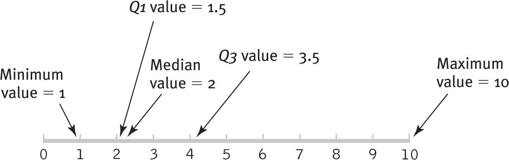
Figure 4-
90
CHECK YOUR LEARNING
Reviewing the Concepts
- The simplest way to measure variability is by using the range, which is calculated by subtracting the lowest score from the highest score.
- Variance and standard deviation both measure the degree to which scores in a distribution vary from the mean. The standard deviation is simply the square root of the variance: It represents the typical deviation of a score from the mean.
- The interquartile range is calculated by subtracting the score at the 25th percentile from the score at the 75th percentile. It communicates the width of the middle 50% of the data.
Clarifying the Concepts
- 4-
6 In your own words, what is variability? - 4-
7 Distinguish the range from the standard deviation. What does each tell us about the distribution?
Calculating the Statistics
- 4-
8 Calculate the range, variance, and standard deviation for the following data sets (the same ones from the section on central tendency).- 10 8 22 5 6 1 19 8 13 12 8
- 122.5 123.8 121.2 125.8 120.2 123.8 120.5 119.8 126.3 123.6
- 0.100 0.866 0.781 0.555 0.222 0.245 0.234
Applying the Concepts
- 4-
9 Final exam week is approaching, and students are not eating as well as usual. Four students were asked how many calories of junk food they had consumed between noon and 10:00 p.m. on the day before an exam. The estimated numbers of nutritionless calories, calculated with the help of a nutritional software program, were 450, 670, 1130, and 1460.- Using the formula, calculate the range for these scores.
- What information can’t you glean from the range?
- Using the formula, calculate variance for these scores.
- Using the formula, calculate standard deviation for these scores.
- If a researcher were interested only in these four students, what symbols would he use for variance and standard deviation, respectively?
- If another researcher hoped to generalize from these four students to all students at the university, what symbols would she use for variance and standard deviation?
Solutions to these Check Your Learning questions can be found in Appendix D.