Testing for Independent Assortment
In some crosses, the genes are obviously linked because there are clearly more nonrecombinant progeny than recombinant progeny. In other crosses, the difference between independent assortment and linkage isn’t as obvious. For example, suppose that we did a testcross for two pairs of genes, such as Aa Bb × aa bb, and observed the following numbers of progeny: 54 Aa Bb, 56 aa bb, 42 Aa bb, and 48 aa Bb. Is this outcome the 1 : 1 : 1 : 1 ratio that we would expect if A and B assorted independently? Not exactly, but it’s pretty close. Perhaps these genes assorted independently and chance produced the slight deviations between the observed numbers and the expected 1 : 1 : 1 : 1 ratio. Alternatively, the genes might be linked, but considerable crossing over might be taking place between them, so that the number of nonrecombinants is only slightly greater than the number of recombinants. How do we distinguish between the role of chance and the role of linkage in producing deviations from the results expected with independent assortment?
We encountered a similar problem in crosses in which genes were unlinked: the problem of distinguishing between deviations due to chance and those due to other factors. We addressed this problem (in Chapter 3) with the chi-square goodness-of-fit test, which helps us evaluate the likelihood that chance alone is responsible for deviations between the numbers of progeny that we observe and the numbers that we expect according to the principles of inheritance. Here, we are interested in a different question: Is the inheritance of alleles at one locus independent of the inheritance of alleles at a second locus? If the answer to this question is yes, then the genes are assorting independently; if the answer is no, then the genes are probably linked.
A possible way to test for independent assortment is to calculate the expected probability of each progeny type, assuming independent assortment, and then use the chi-square goodness-of-fit test to evaluate whether the observed numbers deviate significantly from the expected numbers. With independent assortment, we expect ¼ of each phenotype: ¼ Aa Bb, ¼ aa bb, ¼ Aa bb, and ¼ aa Bb. This expected probability of each genotype is based on the multiplication rule of probability (see Chapter 3). For example, if the probability of Aa is ½ and the probability of Bb is ½, then the probability of Aa Bb is ½ × ½ = ¼. In this calculation, we are making two assumptions: (1) that the probability of each single-locus genotype is ½ and (2) that genotypes at the two loci are inherited independently (½ × ½ = ¼).
Page 126
One problem with this approach is that a significant chi-square value can result from a violation of either assumption. If the genes are linked, then the inheritances of genotypes at the two loci are not independent (assumption 2), and we will get a significant deviation between observed and expected numbers. But we can also get a significant deviation if the probability of each single-locus genotype is not ½ (assumption 1), even when the genotypes are assorting independently. We may obtain a significant deviation, for example, if individuals with one genotype have a lower probability of surviving or if the penetrance of a genotype is not 100%. We could test both assumptions by conducting a series of chi-square tests, first testing the inheritance of genotypes at each locus separately (assumption 1) and then testing for independent assortment (assumption 2). However, a faster method is to test for independence in genotypes with a chi-square test of independence.
THE CHI-SQUARE TEST OF INDEPENDENCE The chi-square test of independence allows us to evaluate whether the segregation of alleles at one locus is independent of the segregation of alleles at another locus without making any assumption about the probability of single-locus genotypes. To illustrate this analysis, let’s examine the results of a cross between German cockroaches, in which yellow body (y) is recessive to brown body (y+) and curved wings (cv) are recessive to straight wings (cv+). A testcross (y+y cv+cv × yy cvcv) produces the progeny shown in Figure 5.9a. If the segregation of alleles at each locus is independent, then the proportions of progeny with y+y and yy genotypes should be the same for cockroaches with genotype cv+cv and for cockroaches with genotype cvcv. The converse is also true: the proportions of progeny with cv+cv and cvcv genotypes should be the same for cockroaches with genotype y+y and for cockroaches with genotype yy.
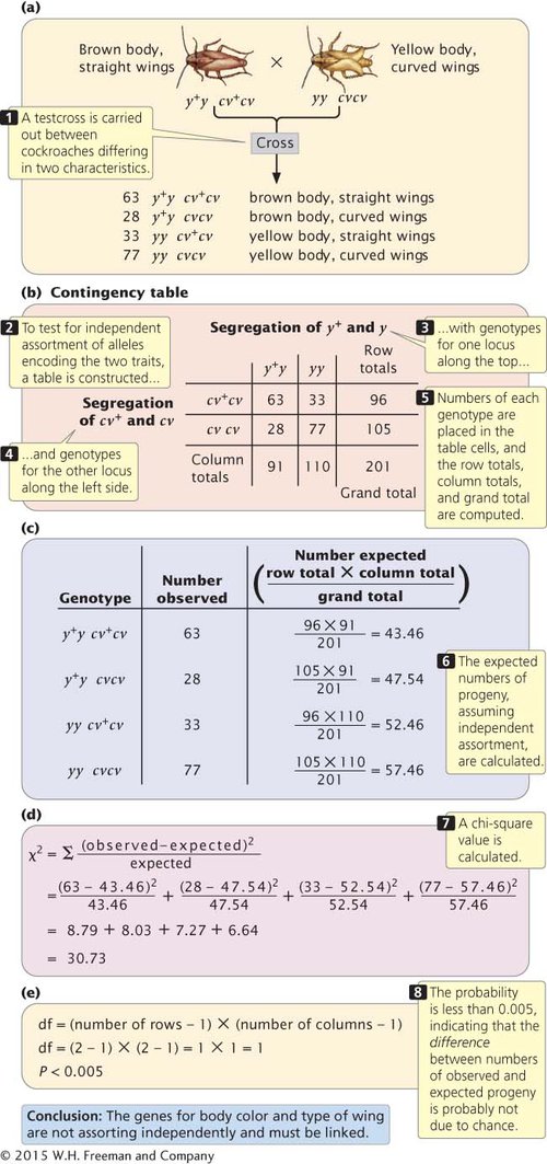
5.9 A chi-square test of independence can be used to determine whether genes at two loci are assorting independently.
Page 127
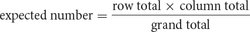
To determine whether the proportions of progeny with genotypes at the two loci are independent, we first construct a table of the observed numbers of progeny, somewhat like a Punnett square, except that we put the genotypes that result from the segregation of alleles at one locus along the top and the genotypes that result from the segregation of alleles at the other locus along the side (Figure 5.9b). Next, we compute the total for each row, the total for each column, and the grand total (the sum of all row totals or the sum of all column totals, which should be the same). These totals will be used to compute the expected values for the chi-square test of independence.
Our next step is to compute the expected values for each combination of genotypes (each cell in the table) under the assumption that the segregation of alleles at the y locus is independent of the segregation of alleles at the cv locus. If the segregation of alleles at each locus is independent, the expected number in each cell can be computed with the following formula:
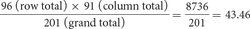
For the cell of the table corresponding to genotype y+y cv+cv (the upper left-hand cell of the table in Figure 5.9b), the expected number is
With the use of this method, we get the expected numbers for each cell that are given in Figure 5.9c.
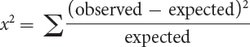
We now calculate a chi-square value by using the same formula that we used for the chi-square goodness-of-fit test in Chapter 3:
Recall that Σ means “sum” and that we are adding together the (observed − expected)2/expected values for each type of progeny. With the observed and expected numbers of cockroaches from the testcross, the calculated chi-square value is 30.73 (Figure 5.9d).
To determine the probability associated with this chi-square value, we need the degrees of freedom. Recall from Chapter 3 that the degrees of freedom are the number of ways in which the observed classes are free to vary from the expected values. In general, for the chi-square test of independence, the degrees of freedom equal the number of rows in the table minus 1 multiplied by the number of columns in the table minus 1 (Figure 5.9e), or
df = (number of rows − 1) × (number of columns − 1)
In our example, there are two rows and two columns, and so the degrees of freedom are
df = (2 − 1) × (2 − 1) = 1 × 1 = 1
Therefore, our calculated chi-square value is 30.73, with 1 degree of freedom. We can use Table 3.4 to find the associated probability. Looking at Table 3.4, we find that our calculated chi-square value is larger than the largest chi-square value given for 1 degree of freedom, which has a probability of 0.005. Thus, our calculated chi-square value has a probability less than 0.005. This very small probability indicates that the genotypes are not in the proportions that we would expect if independent assortment were taking place. Our conclusion, then, is that these genes are not assorting independently and must be linked. As is the case for the chi-square goodness-of-fit test, geneticists generally consider that any chi-square value for the test of independence with a probability less than 0.05 is significantly different from the expected values and is therefore evidence that the genes are not assorting independently.  TRY PROBLEM 10