CONCEPT15.3 Evolution Can Be Measured by Changes in Allele Frequencies
Much of evolution occurs through gradual changes in the relative frequencies of different alleles in a population from one generation to the next. Major genetic changes can also be sudden, as happens when two formerly separated populations merge and hybridize, or when genes within a population are duplicated within the genome (see Concept 15.6). But in most cases, we measure evolution by looking at changes in allele and genotype frequencies in populations over time.
To measure allele frequencies in a population precisely, we would need to count every allele at every locus in every individual in the population. Fortunately, we do not need to make such complete measurements because we can reliably estimate allele frequencies for a given locus by counting alleles in a sample of individuals from the population. The sum of all allele frequencies at a locus is equal to 1, so measures of allele frequency range from 0 to 1.
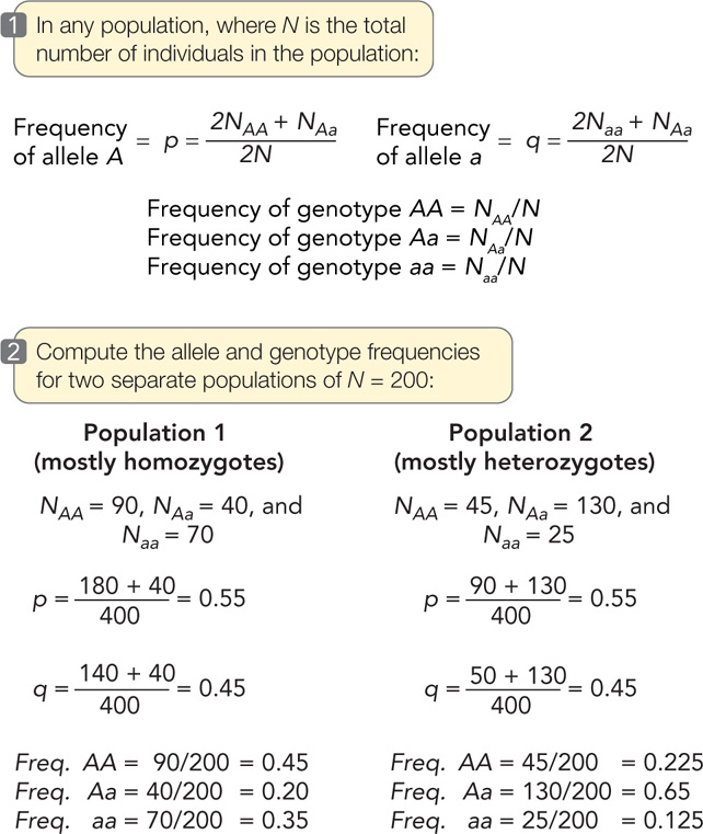
An allele’s frequency is calculated using the following formula:

If only two alleles (we’ll call them A and a) for a given locus are found among the members of a diploid population, those alleles can combine to form three different genotypes: AA, Aa, and aa (see Figure 15.3). A population with more than one allele at a locus is said to be polymorphic (“many forms”) at that locus. Applying the formula above, as shown in FIGURE 15.11, we can calculate the relative frequencies of alleles A and a in a population of N individuals as follows:
- Let NAA be the number that are homozygous for the A allele (AA).
- Let NAa be the number that are heterozygous for the two alleles (Aa).
- Let Naa be the number that are homozygous for the a allele (aa).
Note that NAA + NAa + Naa = N, the total number of individuals in the population, and that the total number of copies of both alleles present in the population is 2N, because each individual is diploid. Each AA individual has two copies of the A allele, and each Aa individual has one copy of the A allele. Therefore the total number of A alleles in the population is 2NAA + NAa. Similarly, the total number of a alleles in the population is 2Naa + NAa. If p represents the frequency of A, and q represents the frequency of a, then
308

and

RESEARCH TOOLS

The calculations in Figure 15.11 demonstrate two important points. First, notice that for each population, p + q = 1, which means that q = 1 − p. So when there are only two alleles at a given locus in a population, we can calculate the frequency of one allele and obtain the second allele’s frequency by subtraction. If there is only one allele at a given locus in a population, its frequency is 1: the population is then monomorphic at that locus, and the allele is said to be fixed.
The second thing to notice is that population 1 (consisting mostly of homozygotes) and population 2 (consisting mostly of heterozygotes) have the same allele frequencies for A and a. Thus they have the same gene pool for this locus. Because the alleles in the gene pool are distributed differently among individuals, however, the genotype frequencies of the two populations differ.
The frequencies of the different alleles at each locus and the frequencies of the different genotypes in a population describe that population’s genetic structure. Allele frequencies measure the amount of genetic variation in a population, whereas genotype frequencies show how a population’s genetic variation is distributed among its members. Other measures, such as the proportion of loci that are polymorphic, are also used to measure variation in populations. With these measurements, it becomes possible to consider how the genetic structure of a population changes or remains the same over generations—that is, to measure evolutionary change.
Evolution will occur unless certain restrictive conditions exist
In 1908, the British mathematician Godfrey Hardy and the German physician Wilhelm Weinberg independently deduced the conditions that must prevail if the genetic structure of a population is to remain the same over time. If the conditions they identified do not exist, then evolution will occur. The resulting principle is known as Hardy–Weinberg equilibrium. Hardy–Weinberg equilibrium describes a model in which allele frequencies do not change across generations and genotype frequencies can be predicted from allele frequencies (FIGURE 15.12). The principles of Hardy–Weinberg equilibrium apply only to sexually reproducing organisms. Several conditions must be met for a population to be at Hardy–Weinberg equilibrium. Note that the following conditions correspond inversely to the five principal processes of evolution (discussed in Concept 15.2):
- There is no mutation. The alleles present in the population do not change, and no new alleles are added to the gene pool.
- There is no selection among genotypes. Individuals with different genotypes have equal probabilities of survival and equal rates of reproduction.
- There is no gene flow. There is no movement of individuals into or out of the population or reproductive contact with other populations.
- Population size is infinite. The larger a population, the smaller will be the effect of genetic drift.
- Mating is random. Individuals do not preferentially choose mates with certain genotypes.

If these idealized conditions hold, two major consequences follow. First, the frequencies of alleles at a locus remain constant from generation to generation. Second, following one generation of random mating, the genotype frequencies occur in the following proportions:

To understand why these consequences are important, start by considering a population that is not in Hardy–Weinberg equilibrium, such as generation I in Figure 15.12. This could occur, for example, if the initial population is founded by migrants from several other populations, thus violating the Hardy–Weinberg assumption of no gene flow. In this example, generation I has more homozygous individuals and fewer heterozygous individuals than would be expected under Hardy–Weinberg equilibrium (a condition known as heterozygote deficiency).
309
Even with a starting population that is not in Hardy–Weinberg equilibrium, we can predict that after a single generation of random mating, and if the other Hardy–Weinberg assumptions are not violated, the allele frequencies will remain unchanged, but the genotype frequencies will return to Hardy–Weinberg expectations. Let’s explore why this is true.
In generation I of Figure 15.12, the frequency of the A allele (p) is 0.55. Because we assume that individuals select mates at random, without regard to their genotype, gametes carrying A or a combine at random—that is, as predicted by the allele frequencies p and q. Thus in this example, the probability that a particular sperm or egg will bear an A allele is 0.55. In other words, 55 out of 100 randomly sampled sperm or eggs will bear an A allele. Because q = 1 − p, the probability that a sperm or egg will bear an a allele is 1 − 0.55 = 0.45.
LINK
You may wish to review the discussion of probability and inheritance in Concept 8.1
To obtain the probability of two A-bearing gametes coming together at fertilization, we multiply the two independent probabilities of their occurrence:
p × p = p2 = (0.55)2 = 0.3025
Therefore 0.3025, or 30.25 percent, of the offspring in generation II will have homozygous genotype AA. Similarly, the probability of two a-bearing gametes coming together is
q × q = q2 = (0.45)2 = 0.2025
which means that 20.25 percent of generation II will have the aa genotype.
There are two ways of producing a heterozygote: an A sperm may combine with an a egg, the probability of which is p × q; or an a sperm may combine with an A egg, the probability of which is q × p. Consequently, the overall probability of obtaining a heterozygote is 2pq, or 0.495. The frequencies of the AA, Aa, and aa genotypes in generation II of Figure 15.12 now meet Hardy–Weinberg expectations, and the frequencies of the two alleles (p and q) have not changed from generation I.
Under the assumptions of Hardy–Weinberg equilibrium, allele frequencies p and q remain constant from generation to generation. If Hardy–Weinberg assumptions are violated and the genotype frequencies in the parental generation are altered (say, by the loss of a large number of AA individuals from the population), then the allele frequencies in the next generation will be altered. However, based on the new allele frequencies, another generation of random mating will be sufficient to restore the genotype frequencies to Hardy–Weinberg equilibrium.
Deviations from Hardy–Weinberg equilibrium show that evolution is occurring
You probably have realized that populations in nature never meet the stringent conditions necessary to be at Hardy–Weinberg equilibrium—which explains why all biological populations evolve. Why, then, is this model considered so important for the study of evolution? There are two reasons. First, the model is useful for predicting the approximate genotype frequencies of a population from its allele frequencies. Second—and crucially—the model allows biologists to evaluate which processes are acting on the evolution of a particular population. The specific patterns of deviation from Hardy–Weinberg equilibrium can help us identify the various processes of evolutionary change.
310
Evolution can be measured by changes in allele frequencies
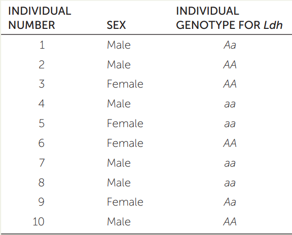
Imagine you have discovered a new population of curly-tailed lizards established on an island after immigrant lizards have arrived from several different source populations during a hurricane. You collect and tabulate genotype data (right) for the lactate dehydrogenase gene (Ldh) for each of the individual lizards. Use the table to answer the following questions.
- Calculate the allele and genotype frequencies of Ldh in this newly founded population.
- Is the population in Hardy–Weinberg equilibrium? If not, which genotypes are over- or underrepresented? Given the population’s history, what is a likely explanation of your answer?
- Under Hardy–Weinberg assumptions, what allele and genotype frequencies do you predict for the next generation?
- Imagine that you are able to continue studying this population and determine the next generation’s actual allele and genotype frequencies. What are some of the principal reasons you might expect the observed allele and genotype frequencies to differ from the Hardy–Weinberg expectations you calculated in question 3?

CHECKpointCONCEPT15.3
- Why is the concept of Hardy–Weinberg equilibrium important even though the assumptions on which it is based are never completely met in nature?
- Although the stringent assumptions of Hardy–Weinberg equilibrium are never met completely in real populations, the genotype frequencies of many populations do not deviate significantly from Hardy–Weinberg expectations. Can you explain why?
- Suppose you examine a population of toads breeding in a single pond and find that heterozygous genotypes at several different loci are present at significantly lower frequencies than predicted by Hardy–Weinberg equilibrium. What are some possible explanations?
Our discussion so far has focused on changes in allele frequencies at a single gene locus. Genes do not exist in isolation, however, but interact with one another (and with the environment) to produce an organism’s phenotype. What effects can these interactions have on selection?