10 Inference for Regression

10.2 Using the Regression Line

One of the most common reasons to fit a line to data is to predict the response to a particular value of the explanatory variable. The method is simple: just substitute the value of into the equation of the line. The least-squares line for predicting log income of entrepreneurs from their years of education (Case 10.1) is

For an EDUC of 16, our least-squares regression equation gives

In terms of inference, there are two different uses of this prediction. First, we can estimate the mean log income in the subpopulation of entrepreneurs with 16 years of education. Second, we can predict the log income of one individual entrepreneur with 16 years of education.

For each use, the actual prediction is the same, . It is the margin of error that is different. Individual entrepreneurs with 16 years of education don’t all have the same log income. Thus, we need a larger margin of error when predicting an individual’s log income than when estimating the mean log income of all entrepreneurs who have 16 years of education.

To emphasize the distinction between predicting a single outcome and estimating the mean of all outcomes in the subpopulation, we use different terms for the two resulting intervals.

To estimate the mean response, we use a confidence interval. This is an ordinary confidence interval for the parameter

The regression model says that is the mean of responses when has the value . It is a fixed number whose value we don’t know.
To estimate an individual response , we use a prediction interval. A prediction interval estimates a single random response rather than a parameter like . The response is not a fixed number. In terms of our example, the model says that different entrepreneurs with the same will have different log incomes.

prediction interval

Fortunately, the meaning of a prediction interval is very much like the meaning of a confidence interval. A 95% prediction interval, like a 95% confidence interval, is right 95% of the time in repeated use. Consider doing the following many times:

511

Draw a sample of observations and one additional observation .
Calculate the 95% prediction interval for and using the observations.

The additional will be in this calculated interval 95% of the time.

Each interval has the usual form

where is the margin of error. The main distinction is that because it is harder to predict for a single observation (random variable) than for the mean of a subpopulation (fixed value), the margin of error for the prediction interval is wider than the margin of error for the confidence interval. Formulas for computing these quantities are given in Section 10.3. For now, we rely on software to do the arithmetic.

Confidence and Prediction Intervals for Regression Response

A level confidence interval for the mean response when takes the value is

Here, is the standard error for estimating a mean response.

A level prediction interval for a single observation on when takes the value is

The standard error for estimating an individual response is larger than the standard error for a mean response to the same .

In both cases, is the value for the density curve with area between and .

Predicting an individual response is an exception to the general fact that regression inference is robust against lack of Normality. The prediction interval relies on Normality of individual observations, not just on the approximate Normality of statistics like the slope and intercept of the least-squares line. In practice, this means that you should regard prediction intervals as rough approximations

EXAMPLE 10.7 Predicting Log Income from Years of Education

entre

CASE 10.1 Alexander Miller is an entrepreneur with years of education. We don’t know his log income, but we can use the data on other entrepreneurs to predict his log income.

Statistical software usually allows prediction of the response for each -value in the data and also for new values of . Here is the output from the prediction option in the Minitab regression command for when we ask for 95% intervals:

FIT	SE FIT	95% CI	95% PI
10.0560	0.167802	(9.72305, 10.3890)	(7.81924, 12.2929)

512

The “Fit” entry gives the predicted log income, 10.0560. This agrees with our hand calculation within rounding error. Minitab gives both 95% intervals. You must choose which one you want. We are predicting a single response, so the prediction interval “95% PI” is the right choice. We are 95% confident that Alexander’s log income lies between 7.81924 and 12.2929. This is a wide range because the data are widely scattered about the least-squares line. The 95% confidence interval for the mean log income of all entrepreneurs with , given as “95% CI,” is much narrower.

Note that Minitab reports only one of the two standard errors. It is the standard error for estimating the mean response, . A graph will help us to understand the difference between the two types of intervals.

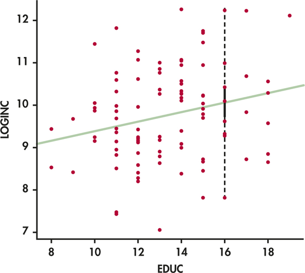
EXAMPLE 10.8 Comparing the Two Intervals

entre

CASE 10.1 Figure 10.13 displays the data, the least-squares line, and both intervals. The confidence interval for the mean is solid. The prediction interval for Alexander’s individual log income level is dashed. You can see that the prediction interval is much wider and that it matches the vertical spread of entrepreneurs’ log incomes about the regression line.

Figure 10.13: FIGURE 10.13 Confidence interval for mean log income (solid) and prediction interval for individual log income (dashed) for an entrepreneur with 16 years of education. Both intervals are centered at the predicted value from the least-squares line, which is for .

Some software packages will graph the intervals for all values of the explanatory variable within the range of the data. With this type of display, it is easy to see the difference between the two types of intervals.

EXAMPLE 10.9 Graphing the Confidence Intervals

CASE 10.1 The confidence intervals for the log income data are graphed in Figure 10.14. For each value of EDUC, we see the predicted value on the solid line and the confidence limits on the dashed curves.

513

Figure 10.14: FIGURE 10.14 95% confidence intervals for mean response for the annual income data.

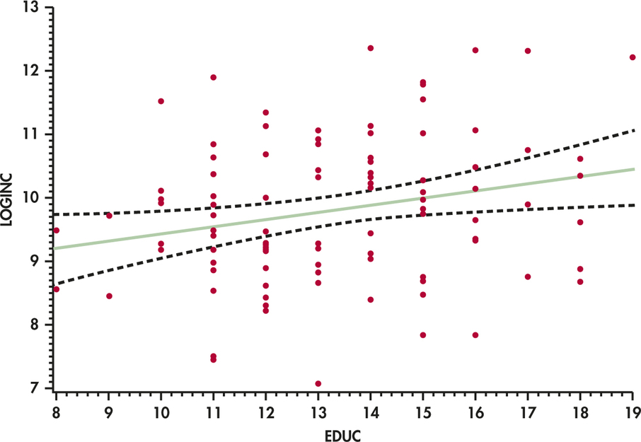
Notice that the in tervals get wider as the values of EDUC move away from the mean of this variable. This phenomenon reflects the fact that we have less information for estimating means that correspond to extreme values of the explanatory variable.

EXAMPLE 10.10 Graphing the Prediction Intervals

CASE 10.1 The prediction intervals for the log income data are graphed in Figure 10.15. As with the confidence intervals, we see the predicted values on the solid line and the prediction limits on the dashed curves.

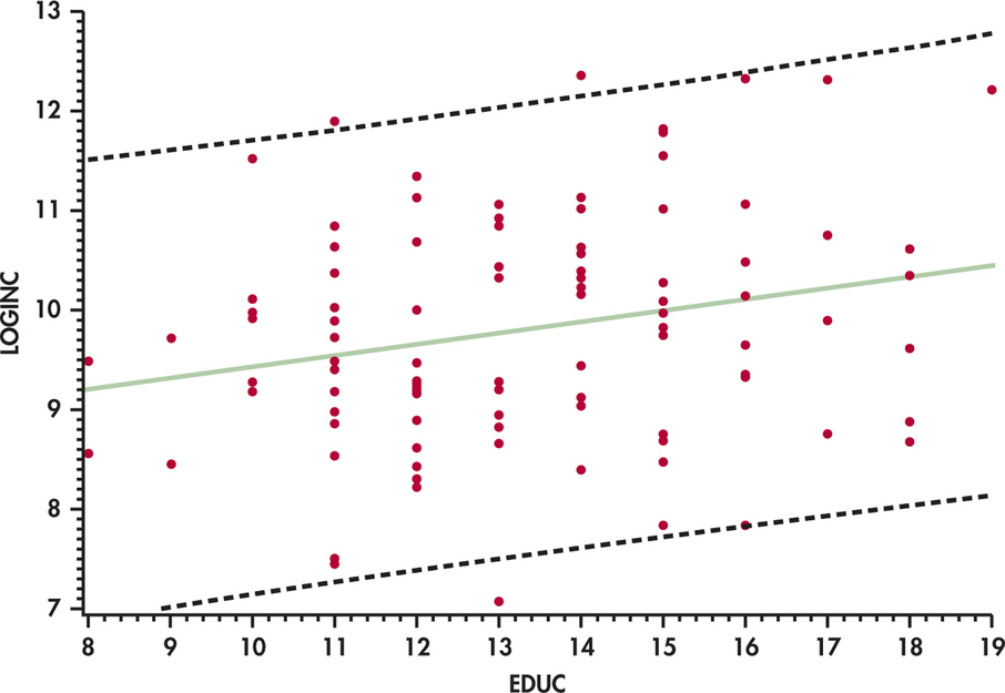
Figure 10.15: FIGURE 10.15 95% prediction intervals for individual response for the annual income data.

514

It is much easier to see the curvature of the confidence limits in Figure 10.14 than the curvature of the prediction limits in Figure 10.15. One reason for this is that the prediction intervals in Figure 10.15 are dominated by the entrepreneur-to entrepreneur variation. Notice that because prediction intervals are concerned with individual predictions, they contain a very large proportion of the data. On the other hand, the confidence intervals are designed to contain mean values and are not concerned with individual observations.

Apply Your Knowledge

Question 10.39

10.39 Predicting the average log income.

In Example 10.7 (pages 511–512) software predicts the mean log income of entrepreneurs with 16 years of education to be . We also see that the standard error of this estimated mean is . These results come from data on 100 entrepreneurs.

Use these facts to verify by hand Minitab’s 95% confidence interval for the mean log income when .
Use the same information to give a 90% confidence interval for the mean log income.

10.39

(a) Using gives (9.72207, 10.38993). (b) For 90% confidence the interval is (9.77678, 10.33522).

Question 10.40

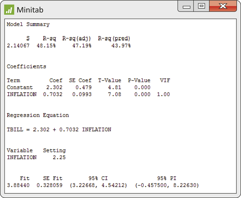
10.40 Predicting the return on Treasury bills.

Table 10.1 (page 498) gives data on the rate of inflation and the percent return on Treasury bills for 55 years. Figures 10.9 and 10.10 analyze these data. You think that next year’s inflation rate will be 2.25%. Figure 10.16 displays part of the Minitab regression output, including predicted values for . The basic output agrees with the Excel results in Figure 10.10.

Verify the predicted value from the equation of the leastsquares line.
What is your 95% interval for predicting next year’s return on Treasury bills?

Figure 10.16: FIGURE 10.16 Minitab output for the regression of the percent return on Treasury bills against the rate of inflation the same year, Exercise 10.40. The output includes predictions of the T-bill return when the inflation rate is 2.25%.

515

Figure 10.17: FIGURE 10.17 The nonlinear model includes these and other relationships between the explanatory variable and the mean response.

Beyond the Basics: Nonlinear Regression

The simple linear regression model assumes that the relationship between theresponse variable and the explanatory variable can be summarized with a straightline. When the relationship is not linear, we can sometimes transform one or both of the variables so that the relationship becomes linear. Exercise 10.39 is an example in which the relationship of log with is linear. In other circumstances, we use models that directly express a curved relationship using parameters that are not just intercepts and slopes. These are nonlinear models.

nonlinear models

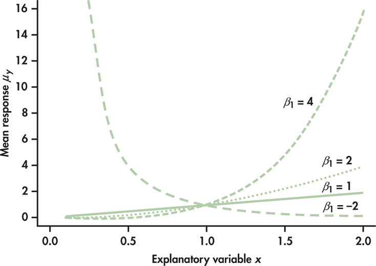
Here is a typical example of a model that involves parameters and in a nonlinear way:

This nonlinear model still has the form

The FIT term describes how the mean response depends on . Figure 10.17 shows the form of the mean response for several values of when . Choosing produces a straight line, but other values of result in a variety of curved relationships.

We cannot write simple formulas for the estimates of the parameters and , but software can calculate both estimates and approximate standard errors for the estimates. If the deviations follow a Normal distribution, we can do inference both on the model parameters and for prediction. The details become more complex, but the ideas remain the same as those we have studied.