11.2 Inference for Multiple Regression
 This page includes Video Technology Manuals
To move from using multiple regression for data analysis to inference in the multiple regression setting, we need to make some assumptions about our data. These assumptions are summarized in the form of a statistical model. As with all the models that we have studied, we do not require that the model be exactly correct. We only require that it be approximately true and that the data do not severely violate the assumptions.

Recall that the simple linear regression model assumes that the mean of the response variable y depends on the explanatory variable x according to a linear equation
μy=β0+β1x
For any fixed value of x, the response y varies Normally around this mean and has a standard deviation σ that is the same for all values of .
In the multiple regression setting, the response variable depends on not one but explanatory variables, which we denote by . The mean response is a linear function of these explanatory variables:
Similar to simple linear regression, this expression is the population regression equation, and the observed ’s vary about their means given by this equation.
population regression equation
Just as we did in simple linear regression, we can also think of this model in terms of subpopulations of responses. The only difference is that each subpopula-tion now corresponds to a particular set of values for all the explanatory variables . The observed ’s in each subpopulation are still assumed to vary Normally with a mean given by the population regression equation and standard deviation that is the same in all subpopulations.
Multiple linear regression model
To form the multiple regression model, we combine the population regression equation with assumptions about the form of the variation of the observations about their mean. We again think of the model in the form
The FIT part of the model consists of the subpopulation mean . The RESIDUAL part represents the variation of the response around its subpopulation mean. That is, the model is
The symbol represents the deviation of an individual observation from its sub-population mean. We assume that these deviations are Normally distributed with mean 0 and an unknown standard deviation that does not depend on the values of the variables.
Multiple Linear Regression Model
The statistical model for multiple linear regression is
for .
The mean response is a linear function of the explanatory variables:
The deviations , are independent and Normally distributed with mean 0 and standard deviation . That is, they are an SRS from the distribution.
The parameters of the model are , and .
The assumption that the subpopulation means are related to the regression coefficients by the equation
implies that we can estimate all subpopulation means from estimates of the ’s. To the extent that this equation is accurate, we have a useful tool for describing how the mean of varies with any collection of ’s.


movies
The Internet Movie Database Pro (IMDbPro) provides movie industry information on both movies and television shows. Can information available soon after a movie’s release be used to predict total U.S. box office revenue? To investigate this, let’s consider an SRS of 43 movies released four to five years ago to guarantee they are no longer in the theaters.10 The response variable is a movie’s total U.S. box office revenue (USRevenue) as of 2014. Among the explanatory variables are the movie’s budget (Budget), opening-weekend revenue (Opening), and how many theaters the movie was in for the opening weekend (Theaters). All dollar amounts are measured in millions of U.S. dollars.
Apply Your Knowledge
Question 11.33
CASE 11.211.33 Look at the data.
Examine the data for total U.S. revenue, budget, opening-weekend revenue, and the number of opening-weekend theaters. That is, use graphs to display the distribution of each variable and the relationships between pairs of variables. Based on your examination, how would you describe the data? Are there any movies you consider to be outliers or unusual in any way? Explain your answer.
11.33
U.S. Revenue, Budget, and Opening are all rightskewed. Opening has a large outlier that may be influential. Theaters is left-skewed. The scatterplots and correlations show that all three have some linear relationship with U.S. revenue, but Opening is the strongest (remember Opening has the outlier also). The correlations show also that there is some linear relationship between the explanatory variables as well.
movies
EXAMPLE 11.12 A Model for Predicting Movie Revenue
CASE 11.2 We want to investigate if a linear model that includes a movie’s budget, opening-weekend revenue, and opening-weekend theater count can forecast total U.S. box office revenue. This multiple regression model has explanatory variables: , , and . Each particular combination of budget, opening-weekend revenue, and opening-weekend theater count defines a particular subpopulation. Our response variable is the U.S. box office revenue as of 2014.
The multiple regression model for the subpopulation mean U.S. box office revenue is
For movies with $35 million budgets that earn $78.23 million in 3700 theaters their first weekend, the model gives the subpopulation mean U.S. box office revenue as
Estimating the parameters of the model
To estimate the mean U.S. box office revenue in Example 11.12, we must estimate the coefficients , , , and . Inference requires that we also estimate the variability of the responses about their means, represented in the model by the standard deviation .
In any multiple regression model, the parameters to be estimated from the data are , and . We estimate these parameters by applying least-squares multiple regression as described in Section 11.1. That is, we view the coefficients in the multiple regression equation
as estimates of the population parameters . The observed variability of the responses about this fitted model is measured by the variance
and the regression standard error
In the model, the parameters and measure the variability of the responses about the population regression equation. It is natural to estimate by and by .
Estimating the Regression Parameters
In the multiple linear regression setting, we use the method of least-squares regression to estimate the population regression parameters.
The standard deviation σ in the model is estimated by the regression standard error
Inference about the regression coefficients
Confidence intervals and significance tests for each of the regression coefficients have the same form as in simple linear regression. The standard errors of the ’s have more complicated formulas, but all are again multiples of . Statistical software does the calculations.
Confidence Intervals and Significance Tests for
A level confidence interval for is
where is the standard error of and is the value for the density curve with area between and .
To test the hypothesis , compute the statistic
In terms of a random variable having the distribution, the -value for a test of against
EXAMPLE 11.13 Predicting U.S. Box Office Revenue
movies
CASE 11.2 In Example 11.12, there are explanatory variables, and we have data on movies. The degrees of freedom for multiple regression are therefore
Statistical software output for this fitted model provides many details of the model’s fit and the significance of the independent variables. Figure 11.11 shows multiple regression outputs from Excel, Minitab, and JMP. You see that the regression equation is
and that the regression standard error is .
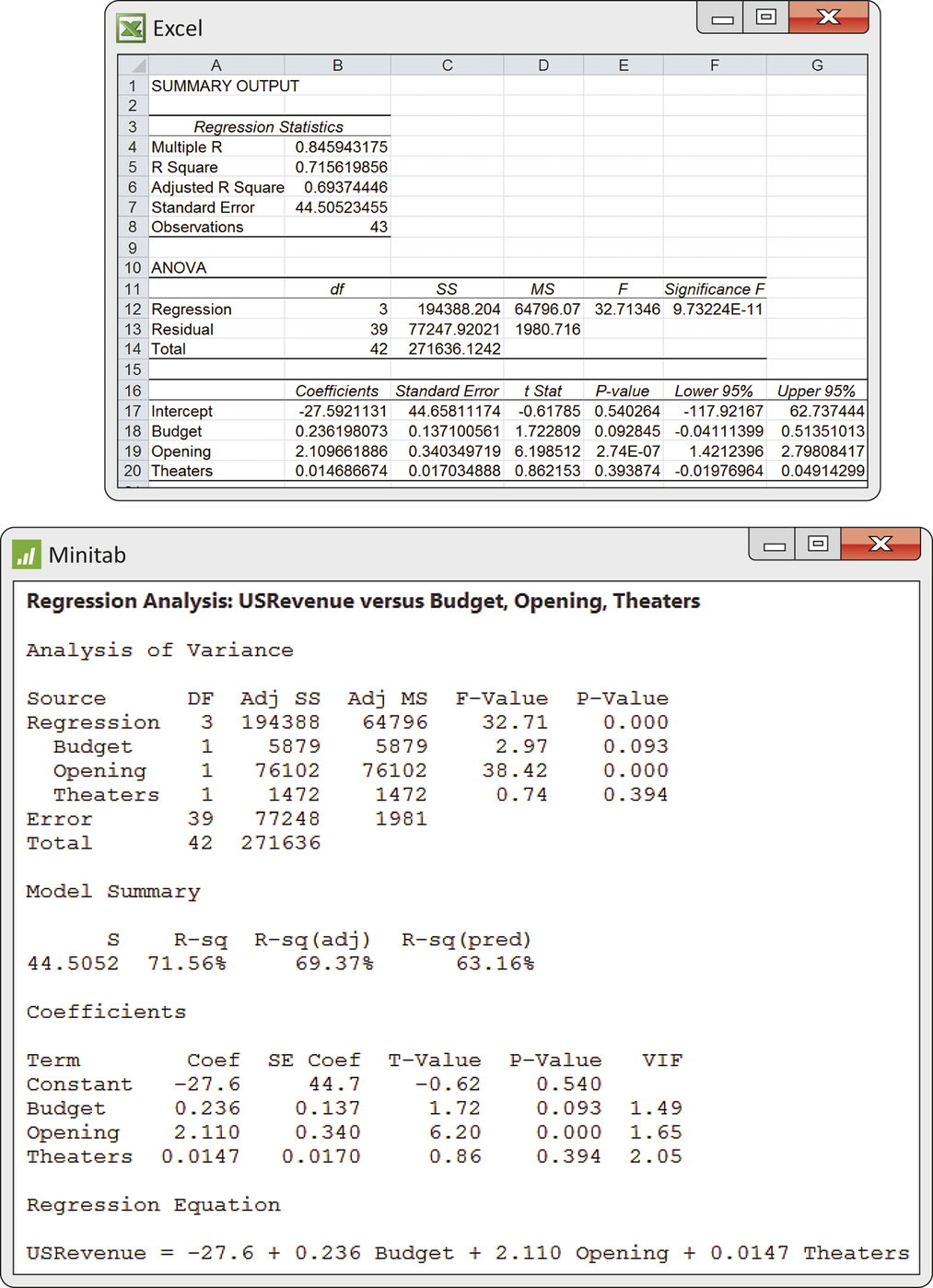
The outputs present the statistic for each regression coefficient and its two-sided -value. For example, the statistic for the coefficient of Opening is 6.20 with a very small -value. The data give strong evidence against the null hypothesis
that the population coefficient for opening-weekend revenue is zero. We would report this result as , , . The software also give the 95% confidence interval for the coefficient . It is (1.42, 2.80). The confidence interval does not include 0, consistent with the fact that the test rejects the null hypothesis at the 5% significance level.

Be very careful in your interpretation of the t tests and confidence intervals for individual regression coefficients. In simple linear regression, the model says that . The null hypothesis says that regression on is of no value for predicting the response , or alternatively, that there is no straight-line relationship between and . The corresponding hypothesis for the multiple regression model of Example 11.13 says that is of no value for predicting y, given that and are also in the model. That’s a very important difference.
The output in Figure 11.11 shows, for example, that the -value for opening-weekend theater count is . We can conclude that the number of theaters does not help predict U.S. box office revenue, given that budget and opening-weekend revenue are available to use for prediction. This does not mean that the opening-weekend theater count cannot help predict U.S. box office revenue. In Exercise 11.33 (page 550) you showed there was a strong positive relationship between the number of theaters and total U.S. revenue, especially when the number of theaters was greater than 2500.
The conclusions of inference about any one explanatory variable in multiple regression depend on what other explanatory variables are also in the model. This is a basic principle for understanding multiple regression. The tests in Example 11.13 show that the opening-weekend theater count does not significantly aid prediction of the U.S. box office revenue if the budget and opening-weekend revenue are also in the model. On the other hand, opening-weekend revenue is highly significant even when the budget and opening-weekend theater count are also in the model.
The interpretation of a confidence interval for an individual coefficient also depends on the other variables in the model, but in this case only if they remain constant. For example, the 95% confidence interval for Opening implies that, given the number of theaters and the budget do not change, a $1 million increase in the opening-weekend revenue results in an expected increase in total U.S. box office revenue somewhere between $1.42 and $2.80 million. While it makes sense for the budget to remain fixed, it may not make sense to keep the number of theaters fixed. The number of theaters and opening-weekend revenue are positively correlated, and it may be very unreasonable to assume that opening revenue can increase this much without the number of theaters also increasing.
Apply Your Knowledge
Question 11.34
CASE 11.211.34 Reading software outputs.
Carefully examine the outputs from the three software packages given in Figure 11.11. Make a table giving the estimated regression coefficient for the movie’s budget (Budget), its standard error, the statistic with degrees of freedom, and the -value as reported by each of the packages. What do you conclude about this coefficient?
Question 11.35
CASE 11.211.35 A simpler model.
In the multiple regression analysis using all three variables, opening-weekend theater count, Theaters, appears to be the least helpful (given that the other two explanatory variables are in the model). Do a new analysis using only the movie’s budget and opening-weekend revenue. Give the estimated regression equation for this analysis and compare it with the analysis using all three explanatory variables. Summarize the inference results for the coefficients. Explain carefully to someone who knows no statistics why the conclusions about budget here and in Figure 11.11 differ.
11.35
. The slope for Budget changed from 0.236 to 0.289, while the slope for Opening changed from 2.110 to 2.264. Additionally, Budget is now significant at the 5% level where it wasn’t before; Opening is still very significant. Conclusions of inference in multiple regression for any explanatory variable depends on what other variables are in the model. In the first model, Budget is interpreted as having Opening and Theaters in the model; once Theaters is removed, the analysis and possible interpretation of Budget will likely change.
movies
Inference about prediction
Inference about the regression coefficients looks much the same in simple and multiple regression, but there are important differences in interpretation. Inference about prediction also looks much the same, and in this case the interpretation is also the same. We may wish to give a confidence interval for the mean response for some specific set of values of the explanatory variables. Or we may want a prediction interval for an individual response for the same set of values.
confidence interval for mean response
prediction interval
The distinction between predicting a mean and individual response is exactly as in simple regression. The prediction interval is again wider because it must allow for the variation of individual responses about the mean. In most software, the commands for prediction inference are the same for multiple and simple regression. The details of the arithmetic performed by the software are, of course, more complicated for multiple regression, but this does not affect interpretation of the output.
What about changes in the model, which we saw can greatly influence inference about the regression coefficients? It is often the case that different models give similar predictions. We expect, for example, that the predictions of U.S. box office revenue from budget and opening-weekend revenue will be about the same as predictions based on budget, opening-weekend revenue, and opening-weekend theater count. Because of this, when prediction is the key goal of a multiple regression, it is common to search for a model that predicts well but does not contain unnecessary predictors. Some refer to this as following the KISS principle.11 In Section 11.3, we discuss some procedures that can be used for this type of search.
Apply Your Knowledge
Question 11.36
CASE 11.211.36 Prediction versus confidence intervals.
For the movie revenue model, would confidence intervals for the mean response or prediction intervals be used more frequently? Explain your answer.
Question 11.37
CASE 11.211.37 Predicting U.S. movie revenue.
The movie Kick-Ass was released during this same time period. It had a budget of $30.0 million and was shown in 3065 theaters, grossing $19.83 million during the first weekend. Use software to construct the following.
- A 95% prediction interval based on the model with all three explanatory variables.
- A 95% prediction interval based on the model using only opening-weekend revenue and budget.
- Compare the two intervals. Do the models give similar predictions and standard errors?
11.37
(a) (−25.5155, 158.2017). (b) (−28.0993, 154.2410). (c) The intervals are quite close; the first model gives a little wider interval because it has a little more standard error for prediction.
movies
ANOVA table for multiple regression
The basic ideas of the regression ANOVA table are the same in simple and multiple regression. ANOVA expresses variation in the form of sums of squares. It breaks the total variation into two parts: the sum of squares explained by the regression equation and the sum of squares of the residuals. The ANOVA table has the same form in simple and multiple regression except for the degrees of freedom, which reflect the number of explanatory variables. Here is the ANOVA table for multiple regression:
| Source | Degrees of freedom | Sum of squares | Mean square | |
|---|---|---|---|---|
| Regression | ||||
| Residual | ||||
| Total |
The brief notation in the table uses, for example, MSE for the residual mean square. This is common notation; the "E’’ stands for "error.’’ Of course, no error has been made. "Error’’ in this context is just a synonym for "residual.’’
The degrees of freedom and sums of squares add, just as in simple regression:
The estimate of the variance for our model is again given by the MSE in the ANOVA table. That is, .
ANOVA F test
The ratio MSR/MSE is again the statistic for the ANOVA test. In simple linear regression, the test from the ANOVA table is equivalent to the two-sided test of the hypothesis that the slope of the regression line is . These two tests are not equivalent in multiple regression.
In the multiple regression setting, the null hypothesis for the test states that all the regression coefficients (with the exception of the intercept) are . One way to write this is
A shorter way to express this hypothesis is
The alternative hypothesis is
The null hypothesis says that none of the explanatory variables helps explain the response, at least when used in the form expressed by the multiple regression equation. The alternative states that at least one of them is linearly related to the response.
This test provides an overall assessment of the model to explain the response. The individual tests assess the importance of a single variable given the presence of the other variables in the model. While looking at the set of individual tests to assess overall model significance may be tempting, it is not recommended because it leads to more frequent incorrect conclusions. The test also better handles situations when there are two or more highly correlated explanatory variables.
As in simple linear regression, large values of give evidence against . When is true, has the distribution. The degrees of freedom for the distribution are those associated with the regression and residual terms in the ANOVA table.
F distributions
The distributions are a family of distributions with two parameters: the degrees of freedom of the mean square in the numerator and denominator of the statistic. The distributions are another of R. A. Fisher’s contributions to statistics and are called in his honor. Fisher introduced statistics for comparing several means. We meet these useful statistics in Chapters 14 and 15.
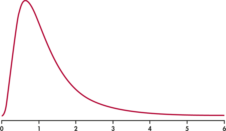
The numerator degrees of freedom are always mentioned first. Interchanging the degrees of freedom changes the distribution, so the order is important. Our brief notation will be for the distribution with degrees of freedom in the numerator and in the denominator. The distributions are not symmetric but are right-skewed. The density curve in Figure 11.12 illustrates the shape. Because mean squares cannot be negative, the statistic takes only positive values, and the distribution has no probability below 0. The peak of the density curve is near 1; values much greater than 1 provide evidence against the null hypothesis.
Tables of critical values are awkward, because a separate table is needed for every pair of degrees of freedom and . Table E in the back of the book gives upper critical values of the distributions for and .
Analysis of Variance Test
In the multiple regression model, the hypothesis
versus
is tested by the analysis of variance statistic
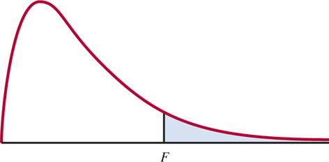
The -value is the probability that a random variable having the distribution is greater than or equal to the calculated value of the statistic.
EXAMPLE 11.14 Test for Movie Revenue Model
movies
CASE 11.2 Example 11.13 (pages 552–553) gives the results of multiple regression analysis for predicting U.S. box office revenue. The statistic is 32.71. The degrees of freedom appear in the ANOVA table. They are 3 and 39. The software packages (see Figure 11.11) report the -value in different forms: Excel, 9.73E-11; Minitab, 0.000; and JMP, <0.0001. Based on all the output, we would report the results as follows: a movie’s budget, opening-weekend revenue, and opening-weekend theater count contain information that can be used to predict the movie’s total U.S. box office revenue (, and 39, ). We’d conclude the same thing with just Excel or JMP output. Based on just Minitab output, we’d only be able to say .
A significant test does not tell us which explanatory variables explain the response. It simply allows us to conclude that at least one of the coefficients is not zero. We may want to refine the model by eliminating some variables that do not appear to be useful (KISS principle). On the other hand, if we fail to reject the null hypothesis, we have found no evidence that any of the coefficients are not zero. In this case, there is little point in attempting to refine the model.
Apply Your Knowledge
Question 11.38
CASE 11.211.38 test for the model without Theaters.
Rerun the multiple regression using the movie’s budget and opening-weekend revenue to predict U.S. box office revenue. Report the statistic, the associated degrees of freedom, and the -value. How do these differ from the corresponding values for the model with the three explanatory variables? What do you conclude?
movies
Squared multiple correlation
For simple linear regression, the square of the sample correlation can be written as the ratio of SSR to SST. We interpret as the proportion of variation in explained by linear regression on . A similar statistic is important in multiple regression.
The Squared Multiple Regression Correlation
The statistic
is the proportion of the variation of the response variable that is explained by the explanatory variables in a multiple linear regression.
Often, is multiplied by 100 and expressed as a percent. The square root of , called the multiple regression correlation coefficient, is the correlation between the observations and the predicted values . Some software provides a scatterplot of this relationship to help visualize the predictive strength of the model.
multiple regression correlation coefficient
EXAMPLE 11.15 for Movie Revenue Model
CASE 11.2 Example 11.13 and Figure 11.11 give the results of multiple regression analysis to predict U.S. box office revenue. The value of the statistic is 0.7156, or 71.56%. Be sure that you can find this statistic in the outputs. We conclude that about 72% of the variation in U.S. box office revenue can be explained by the movies’ budgets, opening-weekend revenues, and opening-weekend theater counts.
The statistic for the multiple regression of U.S. box office revenue on budget, opening-weekend revenue, and opening-weekend theater count is highly significant, . There is strong evidence of a relationship among these three variables and eventual box office revenue. The squared multiple correlation tells us that these variables in this multiple regression model explain about 72% of the variability in box office revenues. The other 28% is represented by the RESIDUAL term in our model and is due to differences among the movies that are not measured by these three variables. For example, these differences might be explained by the movie’s rating, the genre of the movie, and whether the movie is a sequel.
Apply Your Knowledge
Question 11.39
CASE 11.211.39 for different models.
Use each of the following sets of explanatory variables to predict U.S. box office revenue: (a) Budget, Opening; (b) Budget, Theaters; (c) Opening, Theaters; (d) Budget; (e) Opening; (f) Theaters. Make a table giving the model and the value of for each. Summarize what you have found.
11.39
The best model is the model with Budget and Opening with an of 0.7102. Opening and Theater is the second best model with an of 0.6940. The third best model is the one with just Opening with an of 0.6698. The other three models aren’t very good.
| Model | -square |
|---|---|
| Budget, Opening | 0.7102 |
| Budget, Theater | 0.4355 |
| Opening, Theater | 0.694 |
| Budget | 0.26369 |
| Opening | 0.6698 |
| Theater | 0.4009 |
movies
Inference for a collection of regression coefficients
We have studied two different types of significance tests for multiple regression. The test examines the hypothesis that the coefficients for all the explanatory variables are zero. On the other hand, we used tests to examine individual coefficients. (For simple linear regression with one explanatory variable, these are two different ways to examine the same question.)
Often, we are interested in an intermediate setting: does a set of explanatory variables contribute to explaining the response, given that another set of explanatory variables is also available? We formulate such questions as follows: start with the multiple regression model that contains all the explanatory variables and test the hypothesis that a set of the coefficients are all zero. When this set involves more than one explanatory variable, we need to consider an test rather than a set of individual parameter tests.
Test for a Collection of Regression Coefficients
In the multiple regression model with explanatory variables, the hypothesis
versus the hypothesis
is tested by an statistic. The degrees of freedom are and . The -value is the probability that a random variable having the F(, ) distribution is greater than or equal to the calculated value of the statistic.
Some software allows you to directly state and test hypotheses of this form. Here is a way to find the statistic by doing two regression runs.
- Regress on all explanatory variables. Read the -value from the output and call it .
- Then regress on just the variables that remain after removing the variables from the model. Again read the -value and call it . This will be smaller than because removing variables can only decrease .
The test statistic is
with and degrees of freedom.
EXAMPLE 11.16 Do Budget and Opening-Weekend Theater Count Add Predictive Ability?
movies
CASE 11.2 In the multiple regression analysis using all three explanatory variables, opening-weekend revenue (Opening) appears to be the most helpful (given the other two explanatory variables are in the model). A question we might ask is
- Do these other two variables help predict movie revenue, given that opening-weekend revenue is included?
The same question in another form is
- If we start with a model containing all three variables, does removing theater count and budget reduce our ability to predict revenue?
The first regression run includes explanatory variables: Opening, Budget, and Theaters. The for this model is .
Now remove the variables Budget and Theaters and redo the regression with just Opening as the explanatory variable. For this model we get .
The test statistic is
The degrees of freedom are and .
The closest entry in Table E has 2 and 30 degrees of freedom. For this distribution we would need or larger for significance at the 5% level. Thus, . Software gives . Budget and theater count do not contribute significantly to explaining U.S. box office revenue when opening weekend revenue is already in the model.
The hypothesis test in Example 11.16 asks about the coefficients of Budget and Theaters in a model that also contains Opening as an explanatory variable. If we start with a different model, we may get a different answer. For example, we would not be surprised to find that Budget and Theaters help explain movie revenue in a model with only these two explanatory variables. Individual regression coefficients, their standard errors, and significance tests are meaningful only when interpreted in the context of the other explanatory variables in the model.
Apply Your Knowledge
Question 11.40
CASE 11.211.40 Are Budget and Theater useful predictors of USRevenue?
Run the multiple regression to predict movie revenue using all three predictors. Then run the model using only Budget and Theaters.
- The for the second model is 0.4355. Does your work confirm this?
- Make a table giving the Budget and Theaters coefficients and their standard errors, statistics, and -values for both models. Explain carefully how your assessment of the value of these two predictors of movie revenue depends on whether or not opening-weekend revenue is in the model.
movies
Question 11.41
CASE 11.211.41 Is Opening helpful when Budget and Theaters are available?
We saw that Budget and Theaters are not useful in a model that contains the opening-weekend revenue. Now, let’s examine the other version of this question. Does Opening help explain USRevenue in a model that contains Budget and Theaters? Run the models with all three predictors and with only Budget and Theaters. Compare the values of . Perform the test and give its degrees of freedom and -value. Carefully state a conclusion about the usefulness of the predictor Opening when Budget and Theaters are available. Also compare this -test and -value with the test for the coefficient of Opening in Example 11.13.
11.41
The value for all three predictors is 0.7156. The value for just Budget and Theaters is 0.4355. and . Opening does contribute significantly to explaining U.S. box office revenue when Budget and Theaters are already in the model. The conclusion is the same as the test.
movies