16.1 The Wilcoxon Rank Sum Test
 This page includes Video Technology Manuals
Two-sample problems (see Section 7.2) are among the most common in statistics. The most useful nonparametric significance test compares two distributions. Here is an example of this setting.

used
A Midwestern automobile dealership, which we call simply Midwest Auto to preserve confidentiality, has been accused of price discrimination in its selling of used cars. Midwest Auto sells used cars on two different lots. One lot is the standard lot where both new and used cars are sold. This lot is marketed under the name of Midwest Auto. Its other lot exclusively sells used cars. The exclusively used cars lot is marketed under another name than Midwest Auto, which we will call Used Auto.
Customers approaching Midwest Auto who are interested in purchasing a used car are subjected to a credit check. If the dealership assesses the customer as “risky,” then that customer is given only the option to purchase a used car from its subsidiary Used Auto.
Given the customer base for Used Auto is credit risky, car loans offered to these customers come at a higher interest rate. However, the legal matter brought forth to the legal system is that Used Car sells used cars at a higher prices than would have been sold at its Midwest Auto lot. The implication is that there is unfair pricing for a class of consumers. A particular Used Car consumer retained a law firm to pursue a possible class action suit against Midwest Auto.
In the pretrial stage, the Court would not grant opening all records of sales at the two lots. Instead, the Court granted access of data for used cars sold at the two lots during the week of the sale to the plaintiff.
For each used car sold, selling price was compared to the car’s valuation based on the National Automobile Dealers Association (NADA) and converted to a percent. NADA valuations are similar to valuations found in the Black Book or Kelley Blue Book. Data can be viewed as selling price markups relative to NADA valuations. For the week in question, there were 12 used cars sold at Midwest Auto and eight cars sold at Used Auto. Here are the data.
| Lot | Markup % | |||||||||||
| Used Auto | 54.7 | 18.3 | 24.3 | 12.8 | 26.9 | 6.7 | 10.9 | 34.4 | 35.3 | 5.4 | 38.4 | 30.3 |
| Midwest Auto | 13.4 | 24.0 | 19.4 | 8.1 | 3.5 | 5.8 | 7.4 | 5.1 | ||||
Even though the markup percents are all positive here, it is quite possible to get a negative value, which simply means that the consumer purchased the car for less-than book value.
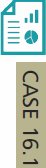
Figure 16.2 is a back-to-back stemplot that compares the markup percents of the 12 Used Auto consumers and the eight Midwest Auto consumers in our sample. The Used Auto distribution has a high outlier, and the Midwest Auto distribution is strongly skewed to the right. If data show neither outliers nor skewness, then two-sample t procedures are fairly robust, even for a total combined sample size of 20 as we have here. However, it is not so clear we can rely on the robustness of the two-sample t test for the data of Case 16.1. We prefer to consider an alternative test that is robust to departures in Normality.

The rank transformation
We first rank all 20 observations together. To do this, arrange them in order from smallest to largest:
| 3.5 | 5.1 | 5.4 | 5.8 | 6.7 | 7.4 | 8.1 | 10.9 | 12.8 | 13.4 |
| 18.3 | 19.4 | 24.0 | 24.3 | 26.9 | 30.3 | 34.4 | 35.3 | 38.4 | 54.7 |
The boldface entries in the list are the sales at the Used Auto lot. The idea of rank tests is to look just at position in this ordered list. To do this, replace each observation by its order, from 1 (smallest) to 20 (largest). These numbers are the ranks:
| Markup % | 3.5 | 5.1 | 5.4 | 5.8 | 6.7 | 7.4 | 8.1 | 10.9 | 12.8 | 13.4 |
| Rank | 1 | 2 | 3 | 4 | 5 | 6 | 7 | 8 | 9 | 10 |
| Markup % | 18.3 | 19.4 | 24.0 | 24.3 | 26.9 | 30.3 | 34.4 | 35.3 | 38.4 | 54.7 |
| Rank | 11 | 12 | 13 | 14 | 15 | 16 | 17 | 18 | 19 | 20 |
Ranks
To rank observations, first arrange them in order from smallest to largest. The rank of each observation is its position in this ordered list, starting with rank 1 for the smallest observation.
Moving from the original observations to their ranks is a transformation of the data, like moving from the observations to their logarithms. The rank transformation retains only the ordering of the observations and makes no other use of their numerical values. Working with ranks allows us to dispense with specific assumptions about the shape of the distribution, such as Normality.
Apply Your Knowledge
Question 16.1
16.1 Numbers of rooms in top spas.
A report of a readers’ poll in Condé Nast Traveler magazine ranked 100 top resort spas.1 Let Group A be the 25 top-ranked spas, and let Group B be the spas ranked 26 to 50. A simple random sample of size 5 was taken from each group, and the number of rooms in each selected spa was recorded. Here are the data.
| Group A | 106 | 145 | 312 | 60 | 49 |
| Group B | 190 | 500 | 1293 | 161 | 225 |
Rank all the observations together and make a list of the ranks for Group A and Group B.
16.1
Group A ranks are 1, 2, 3, 4, 8. Group B ranks are 5, 6, 7, 9, 10.
spas
Question 16.2
16.2 The effect of Animal Kingdom on the result.
Refer to the previous exercise. Disney’s Animal Kingdom in Lake Buena Vista, Florida, with 1293 rooms, was the third spa selected in Group B. Suppose, instead, a different spa, with 540 rooms, had been selected. Replace the observation 1293 in Group B by 540. Use the modified data to make a list of the ranks for Groups A and B combined. What changes?
spas2
The Wilcoxon rank sum test
If Used Car consumers tend to have a higher markup percent relative to Midwest Car consumers, we expect the ranks of the Used Car consumers to be larger than the ranks of the Midwest consumers. Let’s compare the sums of the ranks from the two groups:
| Lot | Sum of ranks |
| Used Auto | 155 |
| Midwest Auto | 55 |
These sums measure how much the ranks of the Used Auto consumers as a group exceed those of the Midwest Auto consumers. In fact, the sum of the ranks from 1 to 20 is always equal to 210, so it is enough to report the sum for one of the two groups. If the sum of the ranks for the Used Auto consumers is 155, the ranks for the Midwest Auto consumers must add to 55 because 155+55=210.
Because there are more Used Auto consumers than Midwest Auto consumers, we would expect the sum of the Used Auto ranks to be greater than the sum of the Midwest Auto ranks if there are no systematic price discrimination differences. But how much greater? Here are the facts we need stated in general form.
The Wilcoxon Rank Sum Test
Draw an SRS of size n1 from one population and draw an independent SRS of size n2 from a second population. There are N observations in all, where N=n1+n2. Rank all N observations. The sum W of the ranks for the first sample is the Wilcoxon rank sum statistic. If the two populations have the same continuous distribution, then W has mean
μW=n1(N+1)2
and standard deviation
σW=√n1n2(N+1)12
The Wilcoxon rank sum test rejects the hypothesis that the two populations have identical distributions when the rank sum W is far from its mean.2
In the used car consumer study of Case 16.1, we want to test
- H0: no difference in distribution of the markup percent for consumers from Midwest Auto and Used Auto lots.
against the one-sided alternative
- Ha: Used Auto consumers are systematically paying a higher markup percent.
Our test statistic is the rank sum W=155 for the Used Auto consumers.
Apply Your Knowledge
Question 16.3
16.3 Hypotheses and test statistic for top spas.
Refer to Exercise 16.1. State appropriate null and alternative hypotheses for this setting and calculate the value of W, the test statistic.
16.3
H0: No difference in distribution of the number of rooms among the 25 top-ranked spas and the spas ranked 26 to 50. Ha: There is a systematic difference in distribution of the number of rooms among the 25 top-ranked spas and the spas ranked 26 to 50. W=18.
spas
Question 16.4
16.4 Effect of Animal Kingdom on the test statistic.
Refer to Exercise 16.2. Using the altered data, state appropriate null and alternative hypotheses and calculate the value of W, the test statistic.
spas2
EXAMPLE 16.1 Perform the Significance Test
CASE 16.1 In Case 16.1, n1=12, n2=8, and there are N=20 observations in all. The sum of ranks for the 12 Used Auto consumers has mean
μW=n1(N+1)2=(12)(21)2=126
and standard deviation
σW=√n1n2(N+1)12=√(12)(8)(21)12=√168=12.961
The observed sum of the ranks, W=155, is higher than the mean by a bit more than two standard deviations since (155−126)/12.961=2.24. It appears that the data support the suspicion that Used Auto consumers are being discriminated against regarding price. The P-value for our one-sided alternative is P(W ≥ 155), the probability that W is at least as large as the value for our data when H0 is true.
To calculate the P-value, P(W ≥ 155), we need to know the sampling distribution of the rank sum W when the null hypothesis is true. This distribution depends on the two sample sizes n1 and n2. Tables are, therefore, a bit unwieldy, though you can find them in handbooks of statistical tables. Most statistical software will give you P-values, as well as carry out the ranking and calculate W. However, some software gives only approximate P-values. You must learn what your software offers.
EXAMPLE 16.2 The P-value
used
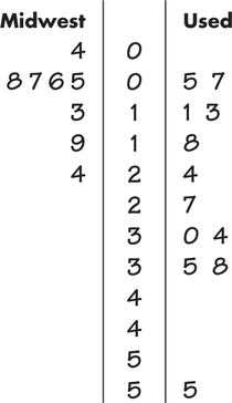
CASE 16.1 Figure 16.3 shows the output from JMP that calculates the exact sampling distribution of W. We see that the sum of the ranks in the first group (Used Auto) is W=155. The reported one-sided P-value is 0.0126. It should be noted that the software computed the P-value based on the sum of ranks for the second group which is 55. It is reporting the probability that the sum of ranks for Midwest Auto consumers is at most as large as 55. This is equivalent to the probability that the sum of ranks for Used Auto consumers is at least as large as 155.
The two-sample t test gives a somewhat more significant result than the Wilcoxon test in Example 16.2 (t=2.80, P=0.006). We hesitate to trust the t test because of the skewness of one sample and the outlier in the other sample along with the fact that the sample sizes are not large.
The Normal approximation
The rank sum statistic W becomes approximately Normal as the two sample sizes increase. We can then form yet another z statistic by standardizing W:
z=W−μWσW=W−n1(N+1)/2√n1n2(N+1)/12
Use standard Normal probability calculations to find P-values for this statistic. Because W takes only whole-number values, the continuity correction can improve the accuracy of the approximation. The idea of continuity correction was first introduced with binomial probability calculations.
EXAMPLE 16.3 The Normal Approximation
CASE 16.1 In our used car consumer example, we are interested in approximating P(W ≥ 155). Continuity correction acts as if the whole number 155 occupies the entire interval from 154.5 to 155.5. We calculate the P-value P(W ≥ 155) as P(W ≥ 154.5) because the value 155 is included in the range whose probability we want. Here is the calculation:
P(W≥154.5)=P(W−μWσW≥154.5−12612.961)=P(Z≥2.1989)=0.0139
The continuity correction gives a result close to the exact value P=0.0126.
We recommend using either the exact distribution (from software or tables) or the continuity correction for the rank sum statistic W. The exact distribution is safer for small samples. As Example 16.3 illustrates, however, the Normal approximation with the continuity correction is often adequate.
EXAMPLE 16.4 Reading Software output
used
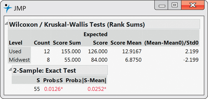
CASE 16.1 Figure 16.4 shows the output for our data from Minitab. Minitab offers only the Normal approximation, and it refers to the Mann-Whitney test.This is an alternative form of the Wilcoxon rank sum test. Minitab gives the approximate onesided P-value as 0.0139 which agrees with our result in Example 16.3.
Mann-Whitney test
Apply Your Knowledge
Question 16.5
16.5 The P-value for top spas.
Refer to Exercises 16.1 and 16.3 (pages 16-5 and 16-6). Find μW, σW, and the standardized rank sum statistic. Then give an approximate P-value using the Normal approximation. What do you conclude?
16.5
μW=27.5, σW=4.7871. We found W=18, so using continuity correction, we get z=−1.88, P-value=0.0301. There is evidence to show a systematic difference in the number of rooms among the 25 top-ranked spas and the spas ranked 26 to 50 at the 5% significance level.
spas
Question 16.6
16.6 The effect of Animal Kingdom on the P-value.
Refer to Exercises 16.2 and 16.4 (pages 16-5 and 16-6). Repeat the analysis in Exercise 16.5 using the altered data.
spas2
What hypotheses do the Wilcoxon test?
Our null hypothesis is that the markup percents of Used Auto consumers and Midwest Auto consumers do not differ systematically. Our alternative hypothesis is that Used Auto consumers’ markup percents are higher. If we are willing to assume that markup percents are Normally distributed, or if we have reasonably large samples, we use the two-sample t test for means. Our hypotheses then become
H0:μ1=μ2Ha:μ1>μ2
When the distributions may not be Normal, we might restate the hypotheses in terms of population medians rather than means:
H0:median1=median2Ha:median1>median2

The Wilcoxon rank sum test does test hypotheses about population medians, but only if an additional assumption is met: both populations must have distributions of the same shape. That is, the density curve for markup percents for Used Auto consumers must look exactly like that for markup percents for Midwest Auto consumers, except that it may slide to a different location on the scale of markup percents. The Minitab output in Figure 16.4 states the hypotheses in terms of population medians (which it denotes as η) and also gives a confidence interval for the difference between the two population medians.
The same-shape assumption is too strict to be reasonable in practice. Recall that our preferred version of the two-sample t test does not require that the two populations have the same standard deviation—that is, it does not make a same-shape assumption. Fortunately, the Wilcoxon test also applies in a much more general and more useful setting. It tests hypotheses that we can state in words as
- H0: The two distributions are the same.
- Ha: One distribution has values that are systematically larger.
systematically larger
Here is a more exact statement of the systematically larger alternative hypothesis. Take X1 to be the markup percent paid by a randomly chosen Used Auto consumer and X2 to be the markup percent paid by a randomly chosen Midwest Auto consumer. These markup percents are random variables. That is, every time we choose a Used Auto consumer at random, the consumer’s markup percent is a value of the variable X1. The probability that a Used Auto consumer’s markup percent is more than 10% is P(X1>10). Similarly, P(X2>10) is the corresponding probability for a randomly chosen Midwest Auto consumer. If the markup percents for Used Auto consumers are “systematically larger” than those of Midwest consumers, getting getting a markup percent greater than 10% should be more likely for Used Auto consumers. That is, we should have
P(X1>10)>P(X2>10)
The alternative hypothesis says that this inequality holds not just for 10% markup but for any markup percent.3
This exact statement of the hypotheses we are testing is a bit awkward. The hypotheses really are “nonparametric” because they do not involve any specific parameter such as the mean or median. If the two distributions do have the same shape, the general hypotheses reduce to comparing medians. Many texts and software outputs state the hypotheses in terms of medians, sometimes ignoring the same-shape requirement. We recommend that you express the hypotheses in words rather than symbols. “Used Auto consumers pay a systematically higher markup percent than Midwest Auto consumers” is easy to understand and is a good statement of the effect that the Wilcoxon test looks for.
Ties
average ranks
The exact distribution for the Wilcoxon rank sum is obtained assuming that all observations in both samples take different values. In theory, with continuous distributions, the probability is 0 that we encounter observations of exactly the same value. Having different values allows us to rank them all. In practice, however, we can encounter observations tied at the same value. What shall we do? The usual practice is to assign all tied values the average of the ranks they occupy. Here is an example with six observations:
| Observation | 10.8 | 13.2 | 23.1 | 23.1 | 29.7 | 30.4 |
| Rank | 1 | 2 | 3.5 | 3.5 | 5 | 6 |
The tied observations occupy the third and fourth places in the ordered list, so they share rank 3.5.
The exact distribution for the Wilcoxon rank sum W applies only to data without ties. Moreover, the standard deviation σW must be adjusted if ties are present. The Normal approximation can be used after the standard deviation is adjusted. Statistical software will detect ties, make the necessary adjustment, and switch to the Normal approximation. In practice, software is required if you want to use rank tests when the data contain tied values.
It is sometimes useful to use rank tests on data that have very many ties because the scale of measurement has only a few values. Here is an example.
fsafety
Vendors of prepared food are very sensitive to the public’s perception of the safety of the food they sell. Food sold at outdoor fairs and festivals may be less safe than food sold in restaurants because it is prepared in temporary locations and often by volunteer help. What do people who attend fairs think about the safety of the food served? One study asked this question of people at a number of fairs in the Midwest:
- How often do you think people become sick because of food they consume prepared at outdoor fairs and festivals?
The possible responses were
- 1=very rarely
- 2=once in a while rarely
- 3=often
- 4=more often than not
- 5=always
In all, 303 people answered the question. Of these, 196 were women and 107 were men. Is there good evidence that men and women differ in their perceptions about food safety at fairs?4
We should first ask if the subjects in Case 16.2 are a random sample of people who attend fairs, at least in the Midwest. The researcher visited 11 different fairs. She stood near the entrance and stopped every 25th adult who passed. Because no personal choice was involved in choosing the subjects, we can reasonably treat the data as coming from a random sample. (As usual, there was some nonresponse, which could create bias.)
Here are the data (variable “sfair” in the associated data file), presented as a two-way table of counts:
| Response | ||||||
|---|---|---|---|---|---|---|
| 1 | 2 | 3 | 4 | 5 | Total | |
| Female | 13 | 108 | 50 | 23 | 2 | 196 |
| Male | 22 | 57 | 22 | 5 | 1 | 107 |
| Total | 35 | 165 | 72 | 28 | 3 | 303 |
Comparing row percents shows that the women in the sample are more concerned about food safety than the men:
| Response | ||||||
| 1 | 2 | 3 | 4 | 5 | Total | |
| Female | 6.6% | 55.1% | 25.5% | 11.7% | 1.0% | 100% |
| Male | 20.6% | 53.3% | 20.6% | 4.7% | 1.0% | 100% |
Is the difference between the genders statistically significant?
We might apply the chi-square test (Chapter 9). It is highly significant (X2=16.120, df=4, P=0.0029). Although the chi-square test answers our general question, it ignores the ordering of the responses and so does not use all of the available information. We would really like to know whether men or women are more concerned about the safety of the food served. This question depends on the ordering of responses from least concerned to most concerned. We can use the Wilcoxon test for the hypotheses:
- H0: men and women do not differ in their responses
- Ha: one gender gives systematically larger responses than the other
The alternative hypothesis is two-sided. Because the responses can take only five values, there are very many ties. All 35 people who chose “very rarely” are tied at 1, and all 165 who chose “once in a while” are tied at 2.
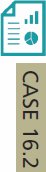
EXAMPLE 16.5 Attitudes Toward Food Sold at Fairs
fsafety
CASE 16.2 Figure 16.5 gives JMP output for the Wilcoxon test. The rank sum for men (using average ranks for ties) is W=14,059.5. The standardized value is z=−3.33, with two-sided P-value P=0.0009. There is very strong evidence of a difference. Women are more concerned than men about the safety of food served at fairs.
With more than 100 observations in each group and no outliers, we might use the two-sample t even though responses take only five values. In fact, the results for Example 16.5 are t=−3.3655 with P=0.0009. The P-value for two-sample t is the same as that for the Wilcoxon test. There is, however, another reason to prefer the rank test in this example. The t statistic treats the response values 1 through 5 as meaningful numbers. In particular, the possible responses are treated as though they are equally spaced. The difference between “very rarely” and “once in a while” is the same as the difference between “once in a while” and “often.” This may not make sense. The rank test, on the other hand, uses only the order of the responses, not their actual values. The responses are arranged in order from least to most concerned about safety, so the rank test makes sense. Some statisticians avoid using t procedures when there is not a fully meaningful scale of measurement.
Apply Your Knowledge
Question 16.7
16.7 CO2 Emissions.
Consider data on CO2 emissions for 2014 compact cars manufactured by the German makers of Mercedes Benz and BMW. For each car, the data are expressed in units of grams of carbon dioxide per kilometer driven. There are many ties among the observations. Arrange the readings in order and assign ranks, assigning all tied values the average of the ranks they occupy.
16.7
There are many tied values; the table below shows the corresponding ranks.
| Type | BMW | Mercedes | BMW | BMW |
|---|---|---|---|---|
| CO2 | 151 | 152 | 161 | 166 |
| Rank | 1 | 2 | 3 | 5 |
| # | 1 | 1 | 1 | 3 |
| Type | BMW | BMW | Mercedes | Mercedes |
| CO2 | 172 | 179 | 182 | 186 |
| Rank | 8.5 | 11.5 | 13 | 14 |
| # | 4 | 2 | 1 | 1 |
| Type | BMW | Mercedes | BMW | BMW |
| CO2 | 189 | 197 | 198 | 200 |
| Rank | 15.5 | 17 | 18.5 | 20.5 |
| # | 2 | 1 | 2 | 2 |
| Type | BMW | BMW | Mercedes | Mercedes |
| CO2 | 202 | 205 | 207 | 209 |
| Rank | 22 | 23.5 | 25 | 26.5 |
| # | 1 | 2 | 1 | 2 |
| Type | Mercedes | BMW | BMW | Mercedes |
| CO2 | 232 | 246 | 255 | 264 |
| Rank | 28 | 29 | 30 | 32 |
| # | 1 | 1 | 1 | 3 |
| Type | Mercedes | Mercedes | ||
| CO2 | 271 | 306 | ||
| Rank | 34 | 35 | ||
| # | 1 | 1 |
gercars
Question 16.8
16.8 Mercedes Benz versus BMW.
Using your ranks from the previous exercise, what is the rank sum W for the Mercedes Benz cars? Using software, is there a significant difference between the CO2 emissions of Mercedes Benz and BMW compact cars?
gercars
Rank versus t tests
The two-sample t procedures are the most common methods for comparing the centers of two populations based on random samples from each. The Wilcoxon rank sum test is a competing procedure that does not start from the condition that the populations have Normal distributions. Both are available in almost all statistical software. How do these two approaches compare in general?
- Moving from the actual data values to their ranks allows us to find an exact sampling distribution for rank statistics such as the Wilcoxon rank sum W when the null hypothesis is true. When our samples are small, are truly random samples from the populations, and show non-Normal distributions of the same shape, the Wilcoxon test is more reliable than the two-sample t test. In most other situations in practice, the robustness of t procedures allows us to obtain reasonably accurate P-values.
- Normal tests compare means and are accompanied by simple confidence intervals for means or differences between means. When we use rank tests to compare medians, we can also give confidence intervals for medians. However, the usefulness of rank tests is clearest in settings when they do not simply compare medians— see the discussion “What hypotheses do the Wilcoxon test?” (page 16-8). Rank methods focus on significance tests, not confidence intervals.
- Inference based on ranks is largely restricted to simple settings. Normal inference extends to methods for use with complex experimental designs and multiple regression, but nonparametric tests do not. We stress Normal inference in part because it leads to more advanced statistics.