4 Probability: The Study of Randomness

4.4 Random Variables

Sample spaces need not consist of numbers. When we toss a coin four times, we can record the outcome as a string of heads and tails, such as HTTH. In statistics, however, we are most often interested in numerical outcomes such as the count of heads in the four tosses. It is convenient to use a shorthand notation: Let be the number of heads. If our outcome is HTTH, then . If the next outcome is TTTH, the value of changes to . The possible values of are 0, 1, 2, 3, and 4. Tossing a coin four times will give one of these possible values. Tossing four more times will give another and probably different value. We call a random variable because its values vary when the coin tossing is repeated.

Random Variable

A random variable is a variable whose value is a numerical outcome of a random phenomenon.

In the preceding coin-tossing example, the random variable is the number of heads in the four tosses.

We usually denote random variables by capital letters near the end of the alphabet, such as or . Of course, the random variables of greatest interest to us are outcomes such as the mean of a random sample, for which we will keep the familiar notation.²² As we progress from general rules of probability toward statistical inference, we will concentrate on random variables.

With a random variable , the sample space just lists the possible values of the random variable. We usually do not mention separately. There remains the second part of any probability model, the assignment of probabilities to events. There are two main ways of assigning probabilities to the values of a random variable. The two types of probability models that result will dominate our application of probability to statistical inference.

210

Discrete random variables

We have learned several rules of probability, but only one method of assigning probabilities: state the probabilities of the individual outcomes and assign probabilities to events by summing over the outcomes. The outcome probabilities must be between 0 and 1 and have sum 1. When the outcomes are numerical, they are values of a random variable. We now attach a name to random variables having probability assigned in this way.

Discrete Random Variable

A discrete random variable has possible values that can be given in an ordered list. The probability distribution of lists the values and their probabilities:

Value of				…
Probability				…

The probabilities must satisfy two requirements:

Every probability is a number between 0 and 1.
The sum of the probabilities is 1; .

Find the probability of any event by adding the probabilities of the particular values that make up the event.

In most of the situations that we will study, the number of possible values is a finite number, . Think about the number of heads in four tosses of a coin. In this case, with taking the possible values of 0, 1, 2, 3, and 4.

However, there are settings in which the number of possible values can be infinite. Think about counting the number of tosses of a coin until you get a head. In this case, the set of possible values for is given by . As another example, suppose represents the number of complaining customers to a retail store during a certain time period. Now, the set of possible values for is given by . In both of these examples, we say that there is a countably infinite number of possible values. Simply defined, countably infinite means that we can correspond each possible outcome to the counting or natural numbers of .

countably infinite

In summary, a discrete random variable either has a finite number of possible values or has a countably infinite number of possible values.

CASE 4.2 Tracking Perishable Demand

Whether a business is in manufacturing, retailing, or service, there is inevitably the need to hold inventory to meet demand on the items held in stock. One of most basic decisions in the control of an inventory management system is the decision of how many items should be ordered to be stocked. Ordering too much leads to unnecessary inventory costs, while ordering too little risks the organization to stock-out situations.

Hospitals have a unique challenge in the inventory management of blood. Blood is a perishable product, and hence a blood inventory management is a trade-off between shortage and wastage. The demand for blood and its components fluctuates. Hospitals routinely track daily blood demand to estimate rates of usage so that they can manage their blood inventory.

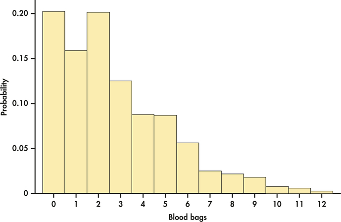
For this case, we consider the daily usage of red blood cells transfusion blood bags collected from a Midwest hospital.²³ These transfusion data are categorized as “new-aged” blood cells, which are used for the most critical patients, such as cancer and immune-deficient patients. If these blood cells are unused by day's end, then they are downgraded to the category of medium-aged blood cells. Here is the distribution of the number of bags used in a day:

211

Bags used	0	1	2	3	4	5	6
Probability	0.202	0.159	0.201	0.125	0.088	0.087	0.056

Bags used	7	8	9	10	11	12
Probability	0.025	0.022	0.018	0.008	0.006	0.003

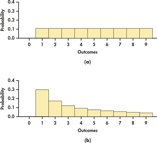
We can use histograms to show probability distributions as well as distributions of data. Figure 4.9 displays the probability histogram of the blood bag probabilities. The height of each bar shows the probability of the outcome at its base. Because the heights are probabilities, they add to 1. As usual, all the bars in a histogram have the same width. So the areas also display the assignment of probability to outcomes. For the blood bag distribution, we can visually see that more than 50% of the distribution is less than or equal to two bags and the distribution is generally skewed to the right. Histograms can also make it easy to quickly compare the two distributions. For example, Figure 4.10 compares the probability model for equally likely random digits (Example 4.13) (pages 186–187) with the model given by Benford's law (Case 4.1) (pages 184–185).

probability histogram

EXAMPLE 4.25 Demand of at Least One Bag?

CASE 4.2 Consider the event that daily demand is at least one bag. In the language of random variables,

The adding of 12 probabilities is a bit of a tedious affair. But there is a much easier way to get at the ultimate probability when we think about the complement rule. The probability of at least one bag demanded is more simply found as follows:

Figure 4.9: FIGURE 4.9 Probability histogram for blood bag demand probabilities. The height of each bar shows the probability assigned to a single outcome.

212

Figure 4.10: FIGURE 4.10 Probability histograms: (a) equally likely random digits 1 to 9; and (b) Benford's law.

With our discussions of discrete random variables in this chapter, it is important to note that our goal is for you to gain a base understanding of discrete random variables and how to work with them. In Chapter 5, we introduce you to two important discrete distributions, known as the binomial and Poisson distributions, that have wide application in business.

Apply Your Knowledge

Question 4.90

4.90 High demand.

CASE 4.2 Refer to Case 4.2 for the probability distribution on daily demand for blood transfusion bags.

What is the probability that the hospital will face a high demand of either 11 or 12 bags? Compute this probability directly using the respective probabilities for 11 and 12 bags.
Now show how the complement rule would be used to find the same probability of part (a).
Consider the calculations of parts (a) and (b) and the calculations of Example 4.25 (page 211). Explain under what circumstances does the use of the complement rule ease computations?

Question 4.91

4.91 How many cars?

Choose an American household at random and let the random variable be the number of cars (including SUVs and light trucks) they own. Here is the probability model if we ignore the few households that own more than five cars:

Number of cars	0	1	2	3	4	5
Probability	0.09	0.36	0.35	0.13	0.05	0.02

Verify that this is a legitimate discrete distribution. Display the distribution in a probability histogram.
Say in words what the event is. Find .
Your company builds houses with two-car garages. What percent of households have more cars than the garage can hold?

4.91

(a) It is a legitimate discrete distribution. (b) The American household owns at least one car. (c) 20%.

213

Figure 4.11: FIGURE 4.11 A spinner that generates a random number between 0 and 1.

Continuous random variables

When we use the table of random digits to select a digit between 0 and 9, the result is a discrete random variable. The probability model assigns probability 1/10 to each of the 10 possible outcomes. Suppose that we want to choose a number at random between 0 and 1, allowing any number between 0 and 1 as the outcome. Software random number generators will do this.

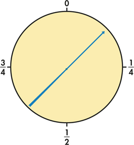
You can visualize such a random number by thinking of a spinner (Figure 4.11) that turns freely on its axis and slowly comes to a stop. The pointer can come to rest anywhere on a circle that is marked from 0 to 1. The sample space is now an interval of numbers:

How can we assign probabilities to events such as ? As in the case of selecting a random digit, we would like all possible outcomes to be equally likely. But we cannot assign probabilities to each individual value of and then sum, because there are infinitely many possible values.

Earlier, we noted that there are situations in which discrete random variables can take on an infinite number of possible values corresponding to the set of counting numbers . However, the infinity associated with the spinner's possible outcomes is a different infinity. There is no way to correspond the infinite number of decimal values in range from 0 to 1 to the counting numbers. We are dealing with the possible outcomes being associated with the real numbers as opposed to the counting numbers. As such, we say here that there is an uncountably infinite number of possible values.

uncountably infinite

In light of these facts, we need to use a new way of assigning probabilities directly to events—as areas under a density curve. Any density curve has area exactly 1 underneath it, corresponding to total probability 1.

EXAMPLE 4.26 Uniform Random numbers

The random number generator will spread its output uniformly across the entire interval from 0 to 1 as we allow it to generate a long sequence of numbers. The results of many trials are represented by the density curve of a uniform distribution.

This density curve appears in red in Figure 4.12. It has height 1 over the interval from 0 to 1, and height 0 everywhere else. The area under the density curve is 1: the area of a rectangle with base 1 and height 1. The probability of any event is the area under the density curve and above the event in question.

uniform distribution

214

Figure 4.12: FIGURE 4.12 Assigning probabilities for generating a random number between 0 and 1, Example 4.26. The probability of any interval of numbers is the area above the interval and under the density curve.

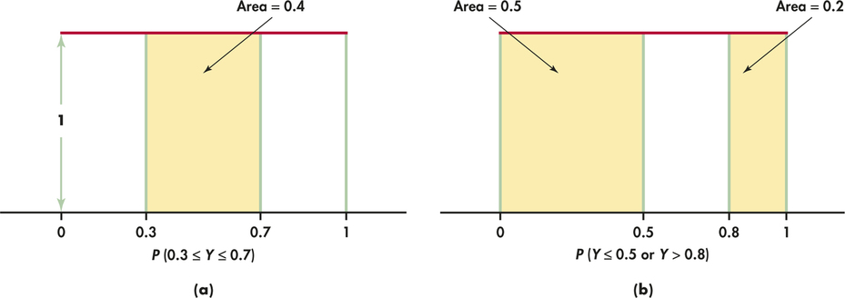
As Figure 4.12(a) illustrates, the probability that the random number generator produces a number between 0.3 and 0.7 is

because the area under the density curve and above the interval from 0.3 to 0.7 is 0.4. The height of the density curve is 1, and the area of a rectangle is the product of height and length, so the probability of any interval of outcomes is just the length of the interval.

Similarly,

Notice that the last event consists of two nonoverlapping intervals, so the total area above the event is found by adding two areas, as illustrated by Figure 4.12(b). This assignment of probabilities obeys all of our rules for probability.

Apply Your Knowledge

Question 4.92

4.92 Find the probability.

For the uniform distribution described in Example 4.26, find the probability that is between 0.2 and 0.7.

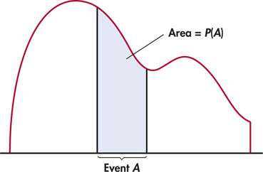
Probability as area under a density curve is a second important way of assigning probabilities to events. Figure 4.13 illustrates this idea in general form. We call in Example 4.26 a continuous random variable because its values are not isolated numbers but an interval of numbers.

Figure 4.13: FIGURE 4.13 The probability distribution of a continuous random variable assigns probabilities as areas under a density curve. The total area under any density curve is 1.

215

Continuous Random Variable

A continuous random variable takes all values in an interval of numbers. The probability distribution of is described by a density curve. The probability of any event is the area under the density curve and above the values of that make up the event.

The probability model for a continuous random variable assigns probabilities to intervals of outcomes rather than to individual outcomes. In fact, all continuous probability distributions assign probability 0 to every individual outcome. Only intervals of values have positive probability. To see that this is true, consider a specific outcome such as in the context of Example 4.26. The probability of any interval is the same as its length. The point 0.8 has no length, so its probability is 0.

Although this fact may seem odd, it makes intuitive, as well as mathematical, sense. The random number generator produces a number between 0.79 and 0.81 with probability 0.02. An outcome between 0.799 and 0.801 has probability 0.002. A result between 0.799999 and 0.800001 has probability 0.000002. You see that as we approach 0.8 the probability gets closer to 0.

To be consistent, the probability of an outcome exactly equal to 0.8 must be 0. Because there is no probability exactly at , the two events and have the same probability. In general, we can ignore the distinction between > and ≥ when finding probabilities for continuous random variables. Similarly, we can also ignore the distinction between < and ≤ in the continuous case. However, when dealing with discrete random variables, we cannot ignore these distinctions. Thus, it is important to be alert as to whether you are dealing with continuous or discrete random variables when doing probability calculations.

Normal distributions as probability distributions

The density curves that are most familiar to us are the Normal curves. Because any density curve describes an assignment of probabilities, Normal distributions are probability distributions. Recall from Section 1.4 (page 44) that is our shorthand for the Normal distribution having mean and standard deviation . In the language of random variables, if has the distribution, then the standardized variable

is a standard Normal random variable having the distribution .

Reminder

standard Normal distribution, p. 46

EXAMPLE 4.27 Tread Life

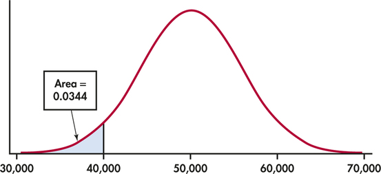
The actual tread life of a 40,000-mile automobile tire has a Normal probability distribution with miles and miles. We say has an distribution. From a manufacturer's perspective, it would be useful to know the probability that a tire fails to meet the guaranteed wear life of 40,000 miles. Figure 4.14 shows this probability as an area under a Normal density curve. You can find it by software or by standardizing and using Table A. From Table A,

The manufacturer should expect to incur warranty costs for about 3.4% of its tires.

216

Figure 4.14: FIGURE 4.14 The Normal distribution with and . The shaded area is , calculated in Example 4.27.

Apply Your Knowledge

Question 4.93

4.93 Normal probabilities.

Example 4.27 gives the Normal distribution for the tread life of a type of tire (in miles). Calculate the following probabilities:

The probability that a tire lasts more than 50,000 miles.
.
.

4.93

(a) 0.5 (b) 0.0344. (c) 0.0344.

We began this chapter with a general discussion of the idea of probability and the properties of probability models. Two very useful specific types of probability models are distributions of discrete and continuous random variables. In our study of statistics, we employ only these two types of probability models.