4.2 Probability Models
 This page includes Statistical Videos
probability model
The idea of probability as a proportion of outcomes in very many repeated trials guides our intuition but is hard to express in mathematical form. A description of a random phenomenon in the language of mathematics is called a probability model. To see how to proceed, think first about a very simple random phenomenon, tossing a coin once. When we toss a coin, we cannot know the outcome in advance. What do we know? We are willing to say that the outcome will be either heads or tails. Because the coin appears to be balanced, we believe that each of these outcomes has probability 1/2. This description of coin tossing has two parts:
- a list of possible outcomes
- a probability for each outcome
This two-part description is the starting point for a probability model. We begin by describing the outcomes of a random phenomenon and then learn how to assign these probabilities ourselves.
Sample spaces
A probability model first tells us what outcomes are possible.
Sample Space
The sample space S of a random phenomenon is the set of all distinct possible outcomes.
The name “sample space” is natural in random sampling, where each possible outcome is a sample and the sample space contains all possible samples. To specify S, we must state what constitutes an individual outcome and then state which outcomes can occur. We often have some freedom in defining the sample space, so the choice of S is a matter of convenience as well as correctness. The idea of a sample space, and the freedom we may have in specifying it, are best illustrated by examples.
EXAMPLE 4.3 Sample Space for Tossing a Coin
Toss a coin. There are only two possible outcomes, and the sample space is
S={heads, tails}
or, more briefly, S={H,T}.
EXAMPLE 4.4 Sample Space for Random digits
Type “=RANDBETWEEN(0,9)” into any Excel cell and hit enter. Record the value of the digit that appears in the cell. The possible outcomes are
S={0, 1, 2, 3, 4, 5, 6, 7, 8, 9}
EXAMPLE 4.5 Sample Space for Tossing a Coin Four Times
Toss a coin four times and record the results. That's a bit vague. To be exact, record the results of each of the four tosses in order. A possible outcome is then HTTH. Counting shows that there are 16 possible outcomes. The sample space S is the set of all 16 strings of four toss results—that is, strings of H's and T's.
Suppose that our only interest is the number of heads in four tosses. Now we can be exact in a simpler fashion. The random phenomenon is to toss a coin four times and count the number of heads. The sample space contains only five outcomes:
S={0, 1, 2, 3, 4}
This example illustrates the importance of carefully specifying what constitutes an individual outcome.
Although these examples seem remote from the practice of statistics, the connection is surprisingly close. Suppose that in conducting a marketing survey, you select four people at random from a large population and ask each if he or she has used a given product. The answers are Yes or No. The possible outcomes—the sample space—are exactly as in Example 4.5 if we replace heads by Yes and tails by No. Similarly, the possible outcomes of an SRS of 1500 people are the same in principle as the possible outcomes of tossing a coin 1500 times. One of the great advantages of mathematics is that the essential features of quite different phenomena can be described by the same mathematical model, which, in our case, is the probability model.
The sample spaces considered so far correspond to situations in which there is a finite list of all the possible values. There are other sample spaces in which, theoretically, the list of outcomes is infinite.
EXAMPLE 4.6 Using Software
Most statistical software has a function that will generate a random number between 0 and 1. The sample space is
S={all numbers between 0 and 1}
This S is a mathematical idealization with an infinite number of outcomes. In reality, any specific random number generator produces numbers with some limited number of decimal places so that, strictly speaking, not all numbers between 0 and 1 are possible outcomes. For example, in default mode, Excel reports random numbers like 0.798249, with six decimal places. The entire interval from 0 to 1 is easier to think about. It also has the advantage of being a suitable sample space for different software systems that produce random numbers with different numbers of digits.
Apply Your Knowledge
Question 4.14
4.14 Describing sample spaces.
In each of the following situations, describe a sample space S for the random phenomenon. In some cases, you have some freedom in your choice of S.
- A new business is started. After two years, it is either still in business or it has closed.
- A student enrolls in a business statistics course and, at the end of the semester, receives a letter grade.Page 181
- A food safety inspector tests four randomly chosen henhouse areas for the presence of Salmonella or not. You record the sequence of results.
- A food safety inspector tests four randomly chosen henhouse areas for the presence of Salmonella or not. You record the number of areas that show contamination.
Question 4.15
4.15 Describing sample spaces.
In each of the following situations, describe a sample space S for the random phenomenon. Explain why, theoretically, a list of all possible outcomes is not finite.
- You record the number of tosses of a die until you observe a six.
- You record the number of tweets per week that a randomly selected student makes.
4.15
(a) Theoretically, it is possible to never roll a 6 because, each time, there is a chance the die will not be a 6. S={1, 2, 3, …}. (b) Theoretically, no matter how many tweets the student made, he or she could make 1 additional tweet, which makes the outcomes infinite. S={0, 1, 2, …}.
A sample space S lists the possible outcomes of a random phenomenon. To complete a mathematical description of the random phenomenon, we must also give the probabilities with which these outcomes occur.
The true long-term proportion of any outcome—say, “exactly two heads in four tosses of a coin”— can be found only empirically, and then only approximately. How then can we describe probability mathematically? Rather than immediately attempting to give “correct” probabilities, let's confront the easier task of laying down rules that any assignment of probabilities must satisfy. We need to assign probabilities not only to single outcomes but also to sets of outcomes.
Event
An event is an outcome or a set of outcomes of a random phenomenon. That is, an event is a subset of the sample space.
EXAMPLE 4.7 Exactly Two Heads in Four Tosses
Take the sample space S for four tosses of a coin to be the 16 possible outcomes in the form HTHH. Then “exactly two heads” is an event. Call this event A. The event A expressed as a set of outcomes is
A={TTHH, THTH, THHT, HTTH, HTHT, HHTT}
In a probability model, events have probabilities. What properties must any assignment of probabilities to events have? Here are some basic facts about any probability model. These facts follow from the idea of probability as “the long-run proportion of repetitions on which an event occurs.”
- Any probability is a number between 0 and 1. Any proportion is a number between 0 and 1, so any probability is also a number between 0 and 1. An event with probability 0 never occurs, and an event with probability 1 occurs on every trial. An event with probability 0.5 occurs in half the trials in the long run.
- All possible outcomes of the sample space together must have probability 1. Because every trial will produce an outcome, the sum of the probabilities for all possible outcomes must be exactly 1.
- If two events have no outcomes in common, the probability that one or the other occurs is the sum of their individual probabilities. If one event occurs in 40% of all trials, a different event occurs in 25% of all trials, and the two can never occur together, then one or the other occurs on 65% of all trials because 40%+25%=65%.
- The probability that an event does not occur is 1 minus the probability that the event does occur. If an event occurs in 70% of all trials, it fails to occur in the other 30%. The probability that an event occurs and the probability that it does not occur always add to 100%, or 1.
Probability rules
Formal probability uses mathematical notation to state Facts 1 to 4 more concisely. We use capital letters near the beginning of the alphabet to denote events. If A is any event, we write its probability as P(A). Here are our probability facts in formal language. As you apply these rules, remember that they are just another form of intuitively true facts about long-run proportions.
Probability Rules
Rule 1. The probability P(A) of any event A satisfies 0≤P(A)≤1.
Rule 2. If S is the sample space in a probability model, then P(S)=1.
Rule 3. Two events A and B are disjoint if they have no outcomes in common and so can never occur together. If A and B are disjoint,
P(A or B)=P(A)+P(B)
This is the addition rule for disjoint events.
Rule 4. The complement of any event A is the event that A does not occur, written as Ac. The complement rule states that
P(Ac)=1-P(A)
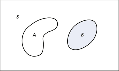
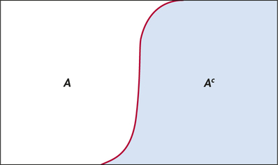
Venn diagram
You may find it helpful to draw a picture to remind yourself of the meaning of complements and disjoint events. A picture like Figure 4.2 that shows the sample space S as a rectangular area and events as areas within S is called a Venn diagram. The events A and B in Figure 4.2 are disjoint because they do not overlap. As Figure 4.3 shows, the complement Ac contains exactly the outcomes that are not in A.
EXAMPLE 4.8 Favorite Vehicle Colors

What is your favorite color for a vehicle? Our preferences can be related to our personality, our moods, or particular objects. Here is a probability model for color preferences.2
| Color | White | Black | Silver | Gray |
| Probability | 0.24 | 0.19 | 0.16 | 0.15 |
| Color | Red | Blue | Brown | Other |
| Probability | 0.10 | 0.07 | 0.05 | 0.04 |
Each probability is between 0 and 1. The probabilities add to 1 because these outcomes together make up the sample space S. Our probability model corresponds to selecting a person at random and asking him or her about a favorite color.
Let's use the probability Rules 3 and 4 to find some probabilities for favorite vehicle colors.
EXAMPLE 4.9 Black or Silver?
What is the probability that a person's favorite vehicle color is black or silver? If the favorite is black, it cannot be silver, so these two events are disjoint. Using Rule 3, we find
P(black or silver)=P(black)+(silver)=0.19+0.16=0.35
There is a 35% chance that a randomly selected person will choose black or silver as his or her favorite color. Suppose that we want to find the probability that the favorite color is not blue.
EXAMPLE 4.10 Use the Complement Rule
To solve this problem, we could use Rule 3 and add the probabilities for white, black, silver, gray, red, brown, and other. However, it is easier to use the probability that we have for blue and Rule 4. The event that the favorite is not blue is the complement of the event that the favorite is blue. Using our notation for events, we have
P(not blue)=1-P(blue)=1-0.07=0.93
We see that 93% of people have a favorite vehicle color that is not blue.
Apply Your Knowledge
Question 4.16
4.16 Red or brown.
Refer to Example 4.8, and find the probability that the favorite color is red or brown.
Question 4.17
4.17 White, black, silver, gray, or red.
Refer to Example 4.8, and find the probability that the favorite color is white, black, silver, gray, or red using Rule 4. Explain why this calculation is easier than finding the answer using Rule 3.
4.17
0.84. This is slightly easier than taking the 5 colors included and adding their probabilities because, here, we can just add the 3 colors that are not included and use the complement rule.
Question 4.18
4.18 Moving up.
An economist studying economic class mobility finds that the probability that the son of a father in the lowest economic class remains in that class is 0.46. What is the probability that the son moves to one of the higher classes?
Question 4.19
4.19 Occupational deaths.
Government data on job-related deaths assign a single occupation for each such death that occurs in the United States. The data on occupational deaths in 2012 show that the probability is 0.183 that a randomly chosen death was a construction worker and 0.039 that it was miner. What is the probability that a randomly chosen death was either construction related or mining related? What is the probability that the death was related to some other occupation?
4.19
By the disjoint rule: 0.222. By the complement rule: 0.778.
Question 4.20
4.20 Grading Canadian health care.
Annually, the Canadian Medical Association uses the marketing research firm Ipsos Canada to measure public opinion with respect to the Canadian health care system. Between July 17 and July 26 of 2013, Ipsos Canada interviewed a random sample of 1000 adults.3 The people in the sample were asked to grade the overall quality of health care services as an A, B, C, or F, where an A is the highest grade and an F is a failing grade. Here are the results:
| Outcome | Probability |
|---|---|
| A | 0.30 |
| B | 0.45 |
| C | ? |
| F | 0.06 |
These proportions are probabilities for choosing an adult at random and asking the person's opinion on the Canadian health care system.
- What is the probability that a person chosen at random gives a grade of C? Why?
- If a “positive” grade is defined as A or B, what is the probability of a positive grade?
Assigning probabilities: Finite number of outcomes
The individual outcomes of a random phenomenon are always disjoint. So, the addition rule provides a way to assign probabilities to events with more than one outcome: start with probabilities for individual outcomes and add to get probabilities for events. This idea works well when there are only a finite (fixed and limited) number of outcomes.
Probabilities in a Finite Sample Space
Assign a probability to each individual outcome. These probabilities must be numbers between 0 and 1 and must have sum 1.
The probability of any event is the sum of the probabilities of the outcomes making up the event.


What is the probability that the leftmost digit (“first digit”) of a multidigit financial number is 9? Many of us would assume the probability to be 1/9. Surprisingly, this is often not the case for legitimately reported financial numbers. It is a striking fact that the first digits of numbers in legitimate records often follow a distribution known as Benford's law. Here it is (note that the first digit can't be 0):
| First digit | 1 | 2 | 3 | 4 | 5 | 6 | 7 | 8 | 9 |
| Proportion | 0.301 | 0.176 | 0.125 | 0.097 | 0.079 | 0.067 | 0.058 | 0.051 | 0.046 |
It is a regrettable fact that financial fraud permeates business and governmental sectors. In a recent 2014 study, the Association of Certified Fraud Examiners (ACFE) estimates that a typical organization loses 5% of revenues each year to fraud.4 ACFE projects a global fraud loss of nearly $4 trillion. Common examples of business fraud include:
- Corporate financial statement fraud: reporting fictitious revenues, understating expenses, artificially inflating reported assets, and so on.
- Personal expense fraud: employee reimbursement claims for fictitious or inflated business expenses (for example, personal travel, meals, etc.).
- Billing fraud: submission of inflated invoices or invoices for fictitious goods or services to be paid to an employee-created shell company.
- Cash register fraud: false entries on a cash register for fraudulent removal of cash.
In all these situations, the individual(s) committing fraud are needing to “invent” fake financial entry numbers. In whatever means the invented numbers are created, the first digits of the fictitious numbers will most likely not follow the probabilities given by Benford's law. As such, Benford's law serves as an important “digital analysis” tool of auditors, typically CPA accountants, trained to look for fraudulent behavior.
Of course, not all sets of data follow Benford's law. Numbers that are assigned, such as Social Security numbers, do not. Nor do data with a fixed maximum, such as deductible contributions to individual retirement accounts (IRAs). Nor, of course, do random numbers. But given a remarkable number of financial-related data sets do closely obey Benford's law, its role in auditing of financial and accounting statements cannot be ignored.
EXAMPLE 4.11 Find Some Probabilities for Benford's Law
CASE 4.1 Consider the events
A={first digit is 5}B={first digit is 3 or less}
From the table of probabilities in Case 4.1,
P(A)=P(5)=0.079P(B)=P(1)+P(2)+P(3)=0.301+0.176+0.125=0.602
Note that P(B) is not the same as the probability that a first digit is strictly less than 3. The probability P(3) that a first digit is 3 is included in “3 or less” but not in “less than 3.”
Apply Your Knowledge
Question 4.21
4.21 Household space heating.
Draw a U.S. household at random, and record the primary source of energy to generate heat for warmth of the household using space-heating equipment. “At random” means that we give every household the same chance to be chosen. That is, we choose an SRS of size 1. Here is the distribution of primary sources for U.S. households:5
| Primary source | Probability |
|---|---|
| Natural gas | 0.50 |
| Electricity | 0.35 |
| Distillate fuel oil | 0.06 |
| Liquefied petroleum gases | 0.05 |
| Wood | 0.02 |
| Other | 0.02 |
- Show that this is a legitimate probability model.
- What is the probability that a randomly chosen U.S. household uses natural gas or electricity as its primary source of energy for space heating?
4.21
(a) 0.50+0.35+0.06+0.05+0.02+0.02=1. (b) 0.85.
Question 4.22
CASE 4.14.22 Benford's law.
Using the probabilities for Benford's law, find the probability that a first digit is anything other than 4.
Question 4.23
CASE 4.14.23 Use the addition rule.
Use the addition rule (Page 182) with the probabilities for the events A and B from Example 4.11 to find the probability of A or B.
4.23
0.681.
EXAMPLE 4.12 Find More Probabilities for Benford's Law
CASE 4.1 Check that the probability of the event C that a first digit is even is
P(C)=P(2)+P(4)+P(6)+P(8)=0.391
Consider again event B from Example 4.11 (page 185), which had an associated probability of 0.602. The probability
P(B or C)=P(1)+P(2)+P(3)+P(4)+P(6)+P(8)=0.817

is not the sum of P(B) and P(C) because events B and C are not disjoint. The outcome of 2 is common to both events. Be careful to apply the addition rule only to disjoint events. In Section 4.3, we expand upon the addition rule given in this section to handle the case of nondisjoint events.
Assigning probabilities: Equally likely outcomes
Assigning correct probabilities to individual outcomes often requires long observation of the random phenomenon. In some circumstances, however, we are willing to assume that individual outcomes are equally likely because of some balance in the phenomenon. Ordinary coins have a physical balance that should make heads and tails equally likely, for example, and the table of random digits comes from a deliberate randomization.
EXAMPLE 4.13 First digits That Are Equally Likely
You might think that first digits in business records are distributed “at random” among the digits 1 to 9. The nine possible outcomes would then be equally likely. The sample space for a single digit is
S={1,2,3,4,5,6,7,8,9}
Because the total probability must be 1, the probability of each of the nine outcomes must be 1/9. That is, the assignment of probabilities to outcomes is
| First digit | 1 | 2 | 3 | 4 | 5 | 6 | 7 | 8 | 9 |
| Probability | 1/9 | 1/9 | 1/9 | 1/9 | 1/9 | 1/9 | 1/9 | 1/9 | 1/9 |
The probability of the event B that a randomly chosen first digit is 3 or less is
P(B)=P(1)+P(2)+P(3)=19+19+19=39=0.333
Compare this with the Benford's law probability in Example 4.11 (page 185). A crook who fakes data by using “random” digits will end up with too few first digits that are 3 or less.
In Example 4.13, all outcomes have the same probability. Because there are nine equally likely outcomes, each must have probability 1/9. Because exactly three of the nine equally likely outcomes are 3 or less, the probability of this event is 3/9. In the special situation in which all outcomes are equally likely, we have a simple rule for assigning probabilities to events.
Equally Likely outcomes
If a random phenomenon has k possible outcomes, all equally likely, then each individual outcome has probability 1/k. The probability of any event A is
P(A)=count of outcomes inAcount of outcomes in S=count of out comes in Ak
Most random phenomena do not have equally likely outcomes, so the general rule for finite sample spaces (page 184) is more important than the special rule for equally likely outcomes.
Apply Your Knowledge
Question 4.24
4.24 Possible outcomes for rolling a die.
A die has six sides with one to six spots on the sides. Give the probability distribution for the six possible outcomes that can result when a fair die is rolled.
Independence and the multiplication rule
Rule 3, the addition rule for disjoint events, describes the probability that one or the other of two events A and B occurs when A and B cannot occur together. Now we describe the probability that both events A and B occur, again only in a special situation. More general rules appear in Section 4.3.
Suppose that you toss a balanced coin twice. You are counting heads, so two events of interest are
A={first toss is a head}B={second toss is a head}
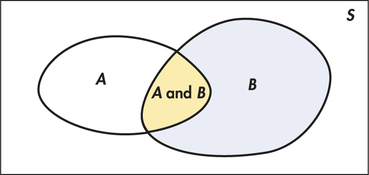
The events A and B are not disjoint. They occur together whenever both tosses give heads. We want to compute the probability of the event {A and B} that both tosses are heads. The Venn diagram in Figure 4.4 illustrates the event {A and B} as the overlapping area that is common to both A and B.
The coin tossing of Buffon, Pearson, and Kerrich described in Example 4.2 makes us willing to assign probability 1/2 to a head when we toss a coin. So,
P(A)=0⋅5P(B)=0⋅5
What is P(A and B)? Our common sense says that it is 1/4. The first coin will give a head half the time and then the second will give a head on half of those trials, so both coins will give heads on 1/2×1/2=1/4 of all trials in the long run. This reasoning assumes that the second coin still has probability 1/2 of a head after the first has given a head. This is true—we can verify it by tossing two coins many times and observing the proportion of heads on the second toss after the first toss has produced a head. We say that the events “head on the first toss” and “head on the second toss” are independent. Here is our final probability rule.
Multiplication Rule for Independent Events
Rule 5. Two events A and B are independent if knowing that one occurs does not change the probability that the other occurs. If A and B are independent,
P(A and B)=P(A)P(B)
This is the multiplication rule for independent events.
Our definition of independence is rather informal. We make this informal idea precise in Section 4.3. In practice, though, we rarely need a precise definition of independence because independence is usually assumed as part of a probability model when we want to describe random phenomena that seem to be physically unrelated to each other.
EXAMPLE 4.14 Determining Independence Using the Multiplication Rule
Consider a manufacturer that uses two suppliers for supplying an identical part that enters the production line. Sixty percent of the parts come from one supplier, while the remaining 40% come from the other supplier. Internal quality audits find that there is a 1% chance that a randomly chosen part from the production line is defective. External supplier audits reveal that two parts per 1000 are defective from Supplier 1. Are the events of a part coming from a particular supplier—say, Supplier 1—and a part being defective independent?
Define the two events as follows:
S1=A randomly chosen part comes from Supplier 1D=A randomly chosen part is defective
We have P(S1)=0.60 and P(D)=0.01. The product of these probabilities is
P(S1)P(D)=(0.60)(0.01)=0.006
However, supplier audits of Supplier 1 indicate that P(S1 and D)=0.002. Given that P(S1 and D) ≠P(S1)P(D), we conclude that the supplier and defective part events are not independent.
The multiplication rule P(A and B)=P(A)P(B) holds if A and B are independent but not otherwise. The addition rule P(A or B)=P(A)+P(B) holds if A and B are disjoint but not otherwise. Resist the temptation to use these simple rules when the circumstances that justify them are not present. You must also be certain not to confuse disjointness and independence. Disjoint events cannot be independent. If A and B are disjoint, then the fact that A occurs tells us that B cannot occur—look back at Figure 4.2 (page 182). Thus, disjoint events are not independent. Unlike disjointness, picturing independence with a Venn diagram is not obvious. A mosaic plot introduced in Chapter 2 provides a better way to visualize independence or lack of it. We will see more examples of mosaic plots in Chapter 9.

Apply Your Knowledge
Question 4.25
4.25 High school rank.
Select a first-year college student at random and ask what his or her academic rank was in high school. Here are the probabilities, based on proportions from a large sample survey of first-year students:
| Rank | Top 20% | Second 20% | Third 20% | Fourth 20% | Lowest 20% |
| Probability | 0.41 | 0.23 | 0.29 | 0.06 | 0.01 |
- Choose two first-year college students at random. Why is it reasonable to assume that their high school ranks are independent?
- What is the probability that both were in the top 20% of their high school classes?
- What is the probability that the first was in the top 20% and the second was in the lowest 20%?
4.25
(a) The rank of one student should not affect the other students’ rank as they likely attended different high schools. (b) 0.1681. (c) 0.0041.
Question 4.26
4.26 College-educated part-time workers?
For people aged 25 years or older, government data show that 34% of employed people have at least four years of college and that 20% of employed people work part-time. Can you conclude that because (0.34)(0.20)=0.068, about 6.8% of employed people aged 25 years or older are college-educated part-time workers? Explain your answer.
Applying the probability rules
If two events A and B are independent, then their complements Ac and Bc are also independent and Ac is independent of B. Suppose, for example, that 75% of all registered voters in a suburban district are Republicans. If an opinion poll interviews two voters chosen independently, the probability that the first is a Republican and the second is not a Republican is (0.75)(1-0.75)=0.1875.
The multiplication rule also extends to collections of more than two events, provided that all are independent. Independence of events A, B, and C means that no information about any one or any two can change the probability of the remaining events. The formal definition is a bit messy. Fortunately, independence is usually assumed in setting up a probability model. We can then use the multiplication rule freely.
By combining the rules we have learned, we can compute probabilities for rather complex events. Here is an example.
EXAMPLE 4.15 False Positives in Job Drug Testing
Job applicants in both the public and the private sector are often finding that preemployment drug testing is a requirement. The Society for Human Resource Management found that 71% of larger organizations (25,000+employees) require drug testing of new job applicants and that 44% of these organizations randomly test hired employees.6 From an applicant's or employee's perspective, one primary concern with drug testing is a “false-positive” result, that is, an indication of drug use when the individual has indeed not used drugs. If a job applicant tests positive, some companies allow the applicant to pay for a retest. For existing employees, a positive result is sometimes followed up with a more sophisticated and expensive test. Beyond cost considerations, there are issues of defamation, wrongful discharge, and emotional distress.
The enzyme multiplied immunoassay technique, or EMIT, applied to urine samples is one of the most common tests for illegal drugs because it is fast and inexpensive. Applied to people who are free of illegal drugs, EMIT has been reported to have false-positive rates ranging from 0.2% to 2.5%. If 150 employees are tested and all 150 are free of illegal drugs, what is the probability that at least one false positive will occur, assuming a 0.2% false positive rate?
It is reasonable to assume as part of the probability model that the test results for different individuals are independent. The probability that the test is positive for a single person is 0.2%, or 0.002, so the probability of a negative result is 1−0.002=0.998 by the complement rule. The probability of at least one false-positive among the 150 people tested is, therefore,
P(at least 1 positive) = 1−P(no positives) = 1−P(150 positives) = 1−0.998150 = 1−0.741=0.259
The probability is greater than 1/4 that at least one of the 150 people will test positive for illegal drugs even though no one has taken such drugs.
Apply Your Knowledge
Question 4.27
4.27 Misleading résumés.
For more than two decades, Jude Werra, president of an executive recruiting firm, has tracked executive résumés to determine the rate of misrepresenting education credentials and/or employment information. On a biannual basis, Werra reports a now nationally recognized statistic known as the “Liars Index.” In 2013, Werra reported that 18.4% of executive job applicants lied on their résumés.7
- Suppose five résumés are randomly selected from an executive job applicant pool. What is the probability that all of the résumés are truthful?
- What is the probability that at least one of five randomly selected résumés has a misrepresentation?
4.27
(a) 0.3618. (b) 0.6382.
Question 4.28
4.28 Failing to detect drug use.
In Example 4.15, we considered how drug tests can indicate illegal drug use when no illegal drugs were actually used. Consider now another type of false test result. Suppose an employee is suspected of having used an illegal drug and is given two tests that operate independently of each other. Test A has probability 0.9 of being positive if the illegal drug has been used. Test B has probability 0.8 of being positive if the illegal drug has been used. What is the probability that neither test is positive if the illegal drug has been used?
Question 4.29
4.29 Bright lights?
A string of holiday lights contains 20 lights. The lights are wired in series, so that if any light fails the whole string will go dark. Each light has probability 0.02 of failing during a three-year period. The lights fail independently of each other. What is the probability that the string of lights will remain bright for a three-year period?
4.29
P(string will remain bright)=P(no lights fail)=(1−0.02)20=0.6676.