4.3 General Probability Rules
 This page includes Video Technology Manuals
 This page includes Statistical Videos
In the previous section, we met and used five basic rules of probability (page 191). To lay the groundwork for probability, we considered simplified settings such as dealing with only one or two events or the making of assumptions that the events are disjoint or independent. In this section, we learn more general laws that govern the assignment of probabilities. We learn that these more general laws of probability allows us to apply probability models to more complex random phenomena.
General addition rules
Probability has the property that if A and B are disjoint events, then P(A or B)=P(A)+P(B). What if there are more than two events or the events are not disjoint? These circumstances are covered by more general addition rules for probability.
Union
The union of any collection of events is the event that at least one of the collection occurs.
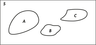
For two events A and B, the union is the event {A or B} that A or B or both occur. From the addition rule for two disjoint events we can obtain rules for more general unions. Suppose first that we have several events—say A, B, and C—that are disjoint in pairs. That is, no two can occur simultaneously. The Venn diagram in Figure 4.5 illustrates three disjoint events. The addition rule for two disjoint events extends to the following law.
Addition Rule for disjoint Events
If events A, B, and C are disjoint in the sense that no two have any outcomes in common, then
P(A or B or C)=P(A)+P(B)+P(C)
This rule extends to any number of disjoint events.
EXAMPLE 4.16 Disjoint Events
Generate a random integer in the range of 10 to 59. What is the probability that the 10's digit will be odd? The event that the 10's digit is odd is the union of three disjoint events. These events are
A={10,11,…,19}B={30,31,…,39}C={50,51,…,59}
In each of these events, there are 10 outcomes out of the 50 possible outcomes. This implies P(A)=P(B)=P(C)=0.2. As a result, the probability that the 10's digit is odd is
P(A or B or C)=P(A)+P(B)+P(C)=0.2+0.2+0.2=0.6
Apply Your Knowledge
Question 4.54
4.54 Probability that sum of dice is a multiple of 4.
Suppose you roll a pair of dice and you record the sum of the dice. What is the probability that the sum is a multiple of 4?
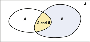
If events A and B are not disjoint, they can occur simultaneously. The probability of their union is then less than the sum of their probabilities. As Figure 4.6 suggests, the outcomes common to both are counted twice when we add probabilities, so we must subtract this probability once. Here is the addition rule for the union of any two events, disjoint or not.
General Addition Rule for Unions of Two Events
For any two events A and B,
P(A or B )=P(A)+P(B)+P(A and B)
If A and B are disjoint, the event {A and B} that both occur has no outcomes in it. This empty event is the complement of the sample space S and must have probability 0. So the general addition rule includes Rule 3, the addition rule for disjoint events.
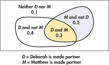
EXAMPLE 4.17 Making Partner
Deborah and Matthew are anxiously awaiting word on whether they have been made partners of their law firm. Deborah guesses that her probability of making partner is 0.7 and that Matthew's is 0.5. (These are personal probabilities reflecting Deborah's assessment of chance.) This assignment of probabilities does not give us enough information to compute the probability that at least one of the two is promoted. In particular, adding the individual probabilities of promotion gives the impossible result 1.2. If Deborah also guesses that the probability that both she and Matthew are made partners is 0.3, then by the general addition rule
P(at least one is promoted)=0.7+0.5-0.3=0.9
The probability that neither is promoted is then 0.1 by the complement rule.
Venn diagrams are a great help in finding probabilities because you can just think of adding and subtracting areas. Figure 4.7 shows some events and their probabilities for Example 4.17. What is the probability that Deborah is promoted and Matthew is not?
The Venn diagram shows that this is the probability that Deborah is promoted minus the probability that both are promoted, 0.7−0.3=0.4. Similarly, the probability that Matthew is promoted and Deborah is not is 0.5−0.3=0.2. The four probabilities that appear in the figure add to 1 because they refer to four disjoint events that make up the entire sample space.
Apply Your Knowledge
Question 4.55
4.55 Probability that sum of dice is even or greater than 8.
Suppose you roll a pair of dice and record the sum of the dice. What is the probability that the sum is even or greater than 8?
4.55
0.6666.
Conditional probability
The probability we assign to an event can change if we know that some other event has occurred. This idea is the key to many applications of probability. Let's first illustrate this idea with labor-related statistics.
Each month the Bureau of Labor Statistics (BLS) announces a variety of statistics on employment status in the United States. Employment statistics are important gauges of the economy as a whole. To understand the reported statistics, we need to understand how the government defines “labor force.” The labor force includes all people who are either currently employed or who are jobless but are looking for jobs and are available for work. The latter group is viewed as unemployed. People who have no job and are not actively looking for one are not considered to be in the labor force. There are a variety of reasons for people not to be in the labor force, including being retired, going to school, having certain disabilities, or being too discouraged to look for a job.
EXAMPLE 4.18 Labor Rates
Averaged over the year 2013, the following table contains counts (in thousands) of persons aged 16 and older in the civilian population, classified by gender and employment status:15
| Gender | Employed | Unemployed | Not in labor force | Civilian population |
|---|---|---|---|---|
| Men | 76,353 | 6,314 | 35,889 | 118,556 |
| Women | 67,577 | 5,146 | 54,401 | 127,124 |
| Total | 143,930 | 11,460 | 90,290 | 245,680 |
The BLS defines the total labor force as the sum of the counts on employed and unemployed. In turn, the total labor force count plus the count of those not in the labor force equals the total civilian population. Depending on the base (total labor force or civilian population), different rates can be computed. For example, the number of people unemployed divided by the total labor force defines the unemployment rate, while the total labor force divided by the civilian population defines labor participation rate.
Randomly choose a person aged 16 or older from the civilian population. What is the probability that person is defined as labor participating? Because “choose at random” gives all 245,680,000 such persons the same chance, the probability is just the proportion that are participating. In thousands,
P(participating)=143,930+11,460245,680=0.632
This calculation does not assume anything about the gender of the person. Suppose now we are told that the person chosen is female. The probability that the person participates, given the information that the person is female, is
P(participating | females) = 67,577+5,146127,124=0.572
The new notation P(B | A) is a conditional probability. That is, it gives the probability of one event (person is labor participating) under the condition that we know another event (person is female). You can read the bar | as “given the information that.”
conditional probability
Apply Your Knowledge
Question 4.56
4.56 Men labor participating.
Refer to Example 4.18. What is the probability that a person is labor participant given the person is male?

Do not confuse the probabilities of P(B | A) and P(A and B). They are generally not equal. Consider, for example, that the computed probability of 0.572 from Example 4.18 is not the probability that a randomly selected person from the civilian population is female and labor participating. Even though these probabilities are different, they are connected in a special way. Find first the proportion of the civilian population who are women. Then, out of the female population, find the proportion who are labor participating. Multiply the two proportions. The actual proportions from Example 4.18 are
P(female and participating)=P(female)×P(participating | female)=(127,124245,680)(0.572)=0.296
We can check if this is correct by computing the probability directly as follows:
P(female and participating)=67,577+5,146245,680=0.296
We have just discovered the general multiplication rule of probability.
Multiplication Rule
The probability that both of two events A and B happen together can be found by
P(A and B)=P(A)P(B | A)
Here P(B | A) is the conditional probability that B occurs, given the information that A occurs.
EXAMPLE 4.19 Downloading Music from the Internet
The multiplication rule is just common sense made formal. For example, suppose that 29% of Internet users download music files, and 67% of downloaders say they don't care if the music is copyrighted. So the percent of Internet users who download music (event A) and don't care about copyright (event B) is 67% of the 29% who download, or
(0.67)(0.29)=0.1943=19.43%
The multiplication rule expresses this as
P(A and B)=P(A)×P(B | A)=(0.29)(0.67)=0.1943
Apply Your Knowledge
Question 4.57
4.57 Focus group probabilities.
A focus group of 15 consumers has been selected to view a new TV commercial. Even though all of the participants will provide their opinion, two members of the focus group will be randomly selected and asked to answer even more detailed questions about the commercial. The group contains seven men and eight women. What is the probability that the two chosen to answer questions will both be women?
4.57
0.2667.
Question 4.58
4.58 Buying from Japan.
Functional Robotics Corporation buys electrical controllers from a Japanese supplier. The company's treasurer thinks that there is probability 0.4 that the dollar will fall in value against the Japanese yen in the next month. The treasurer also believes that if the dollar falls, there is probability 0.8 that the supplier will demand renegotiation of the contract. What probability has the treasurer assigned to the event that the dollar falls and the supplier demands renegotiation?
If P(A) and P(A and B) are given, we can rearrange the multiplication rule to produce a definition of the conditional probability P(B | A) in terms of unconditional probabilities.
Definition of Conditional Probability
When P(A)>0, the conditional probability of B given A is
P(B | A)=P(A and B)P(A)
Be sure to keep in mind the distinct roles in P(B | A) of the event B whose probability we are computing and the event A that represents the information we are given. The conditional probability P(B | A) makes no sense if the event A can never occur, so we require that P(A)>0 whenever we talk about P(B | A).
EXAMPLE 4.20 College Students
Here is the distribution of U.S. college students classified by age and full-time or part-time status:
| Age (years) | Full-time | Part-time |
| 15 to 19 | 0.21 | 0.02 |
| 20 to 24 | 0.32 | 0.07 |
| 25 to 39 | 0.10 | 0.10 |
| 30 and over | 0.05 | 0.13 |
Let's compute the probability that a student is aged 15 to 19, given that the student is full-time. We know that the probability that a student is full-time and aged 15 to 19 is 0.21 from the table of probabilities. But what we want here is a conditional probability, given that a student is full-time. Rather than asking about age among all students, we restrict our attention to the subpopulation of students who are full-time. Let
A=the student is a full-time studentB=the student is between 15 and 19 years of age
Our formula is
P(B | A)=P(A and B)P(A)
We read P(A and B)=0.21 from the table as mentioned previously. What about P(A)? This is the probability that a student is full-time. Notice that there are four groups of students in our table that fit this description. To find the probability needed, we add the entries:
P(A)=0.21+0.32+0.10+0.05=0.68
We are now ready to complete the calculation of the conditional probability:
P(B | A)=P(A and B)P(A)=0.210.68=0.31
The probability that a student is 15 to 19 years of age, given that the student is fulltime, is 0.31.
Here is another way to give the information in the last sentence of this example: 31% of full-time college students are 15 to 19 years old. Which way do you prefer?
Apply Your Knowledge
Question 4.59
4.59 What rule did we use?
In Example 4.20, we calculated P(A). What rule did we use for this calculation? Explain why this rule applies in this setting.
4.59
Rule 3. Addition rule for disjoint events. It applies in this setting because a student can’t be in more than one age group, so the four age groups are disjoint.
Question 4.60
4.60 Find the conditional probability.
Refer to Example 4.20. What is the probability that a student is part-time, given that the student is 15 to 19 years old? Explain in your own words the difference between this calculation and the one that we did in Example 4.20.
General multiplication rules
The definition of conditional probability reminds us that, in principle, all probabilities—including conditional probabilities—can be found from the assignment of probabilities to events that describe random phenomena. More often, however, conditional probabilities are part of the information given to us in a probability model, and the multiplication rule is used to compute P(A and B). This rule extends to more than two events.
The union of a collection of events is the event that any of them occur. Here is the corresponding term for the event that all of them occur.
Intersection
The intersection of any collection of events is the event that all the events occur.
To extend the multiplication rule to the probability that all of several events occur, the key is to condition each event on the occurrence of all the preceding events. For example, the intersection of three events A, B, and C has probability
P(A and B and C)=P(A)P(B | A)P(C | A and B)
EXAMPLE 4.21 Career in Big Business: NFL
Worldwide, the sports industry has become synonymous with big business. It has been estimated by the United Nations that sports account for nearly 3% of global economic activity. The most profitable sport in the world is professional football under the management of the National Football League (NFL).16 With multi-million-dollar signing contracts, the economic appeal of pursuing a career as a professional sports athlete is unquestionably strong. But what are the realities? Only 6.5% of high school football players go on to play at the college level. Of these, only 1.2% will play in the NFL.17 About 40% of the NFL players have a career of more than three years. Define these events for the sport of football:
A={competes in college}B={competes in the NFL}C={has an NFL career longer than 3 years}
What is the probability that a high school football player competes in college and then goes on to have an NFL career of more than three years? We know that
P(A)=0.065P(B | A)=0.012P(C | A and B)=0.4
The probability we want is, therefore,
P(A and B and C)=P(A)P(B | A)P(C | A and B)=0.065×0.012×0.40=0.00031
Only about three of every 10,000 high school football players can expect to compete in college and have an NFL career of more than three years. High school football players would be wise to concentrate on studies rather than unrealistic hopes of fortune from pro football.
Tree diagrams
In Example 4.21, we investigated the likelihood of a high school football player going on to play collegiately and then have an NFL career of more than three years. The sports of football and basketball are unique in that players are prohibited from going straight into professional ranks from high school. Baseball, however, has no such restriction. Some baseball players might make the professional rank through the college route, while others might ultimately make it coming out of high school, often with a journey through the minor leagues.
The calculation of the probability of a baseball player becoming a professional player involves more elaborate calculation than the football scenario. We illustrate with our next example how the use of a tree diagram can help organize our thinking.
tree diagram
EXAMPLE 4.22 How Many Go to MLB?
For baseball, 6.8% of high school players go on to play at the college level. Of these, 9.4% will play in Major League Baseball (MLB).18 Borrowing the notation of Example 4.21, the probability of a high school player ultimately playing professionally is P(B). To find P(B), consider the tree diagram shown in Figure 4.8.
Each segment in the tree is one stage of the problem. Each complete branch shows a path that a player can take. The probability written on each segment is the conditional probability that a player follows that segment given that he has reached the point from which it branches. Starting at the left, high school baseball players either do or do not compete in college. We know that the probability of competing in college is P(A)=0.068, so the probability of not competing is P(Ac)=0.932. These probabilities mark the leftmost branches in the tree.
Conditional on competing in college, the probability of playing in MLB is P(B | A)=0.094. So the conditional probability of not playing in MLB is
P(Bc|A)=1-P(B | A)=1-0.094=0.906
These conditional probabilities mark the paths branching out from A in Figure 4.8.
The lower half of the tree diagram describes players who do not compete in college (Ac). For baseball, in years past, the majority of destined professional players did not take the route through college. However, nowadays it is relatively unusual for players to go straight from high school to MLB. Studies have shown that the conditional probability that a high school athlete reaches MLB, given that he does not compete in college, is P(B | Ac)=0.002.19 We can now mark the two paths branching from Ac in Figure 4.8.
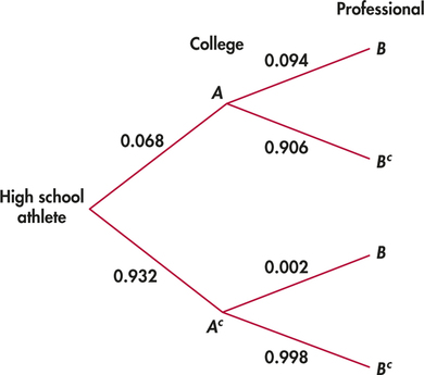
There are two disjoint paths to B (MLB play). By the addition rule, P(B) is the sum of their probabilities. The probability of reaching B through college (top half of the tree) is
P(A and B)=P(A)P(B | A)=0.068×0.094=0.006392
The probability of reaching B without college is
P(Ac and B)=P(Ac)P(B | Ac)=0.932×0.002=0.001864
The final result is
P(B)=0.006392+0.001864=0.008256
About eight high school baseball players out of 1000 will play professionally. Even though this probability is quite small, it is comparatively much greater than the chances of making it to the professional ranks in basketball and football.
It takes longer to explain a tree diagram than it does to use it. Once you have understood a problem well enough to draw the tree, the rest is easy. Tree diagrams combine the addition and multiplication rules. The multiplication rule says that the probability of reaching the end of any complete branch is the product of the probabilities written on its segments. The probability of any outcome, such as the event B that a high school baseball player plays in MLB, is then found by adding the probabilities of all branches that are part of that event.
Apply Your Knowledge
Question 4.61
4.61 Labor rates.
Refer to the labor data in Example 4.18 (page 197). Draw a tree diagram with the first-stage branches being gender. Then, off the gender branches, draw two branches as the outcomes being “labor force participating” versus “not in the labor force.” Show how the tree would be used to compute the probability that a randomly chosen person is labor force participating.
4.61
P(labor force participant)=P(labor force partcipant and male)+P(labor force participant and female)=P(labor force participant male)P(male)+P(labor force participant|female)P(female)=0.6973(0.4826)+0.5721(0.5174)=0.6325.
Bayes's rule
There is another kind of probability question that we might ask in the context of studies of athletes. Our earlier calculations look forward toward professional sports as the final stage of an athlete's career. Now let's concentrate on professional athletes and look back at their earlier careers.
EXAMPLE 4.23 Professional Athletes' Pasts
What proportion of professional athletes competed in college? In the notation of Examples 4.21 and 4.22, this is the conditional probability P(A | B). Before we compute this probability, let's take stock of a few facts. First, the multiplication rule tells us
P(A and B)=P(A)P(B | A)
We know the probabilities P(A) and P(Ac) that a high school baseball player does and does not compete in college. We also know the conditional probabilities P(B | A) and P(B | Ac) that a player from each group reaches MLB. Example 4.22 shows how to use this information to calculate P(B). The method can be summarized in a single expression that adds the probabilities of the two paths to B in the tree diagram:
P(B)=P(A)P(B | A)+P(Ac)P(B | Ac)
Combining these facts, we can now make the following computation:
P(A | B)=P(A and B)P(B)=P(A)P(B | A)P(A)P(B | A)+P(Ac)P(B | Ac)=0.068×0.0940.068×0.094+0.932×0.002=0.774
About 77% of MLB players competed in college.
In calculating the “reverse” conditional probability of Example 4.23, we had two disjoint events in A and Ac whose probabilities add to exactly 1. We also had the conditional probabilities of event B given each of the disjoint events. More generally, there can be applications in which we have more than two disjoint events whose probabilities add up to 1. Put in general notation, we have another probability law.
Bayes's Rule
Suppose that A1,A2,…,Ak are disjoint events whose probabilities are not 0 and add to exactly 1. That is, any outcome is in exactly one of these events. Then, if B is any other event whose probability is not 0 or 1,
P(Ai|B)=P(B | Ai)P(Ai)P(B | A1)P(A1)+P(B | A2)P(A2)+⋯+P(B | Ak)P(Ak)
The numerator in Bayes's rule is always one of the terms in the sum that makes up the denominator. The rule is named after Thomas Bayes, who wrestled with arguing from outcomes like event B back to the Ai in a book published in 1763. Our next example utilizes Bayes's rule with several disjoint events.
EXAMPLE 4.24 Credit Ratings
Corporate bonds are assigned a credit rating that provides investors with a guide of the general creditworthiness of a corporation as a whole. The most well-known credit rating agencies are Moody's, Standard & Poor's, and Fitch. These rating agencies assign a letter grade to the bond issuer. For example, Fitch uses the letter classifications of AAA, AA, A, BBB, BB, B, CCC, and D. Over time, the credit ratings of the corporation can change. Credit rating specialists use the terms of “credit migration” or “transition rate” to indicate the probability of a corporation going from letter grade to letter grade over some particular span of time. For example, based on a large amount of data from 1990 to 2013, Fitch estimates that the five-year transition rates to be graded AA in the fifth year based on each of the current (“first year”) grades to be:20
| Current rating | AA (in 5th year) |
|---|---|
| AAA | 0.2283 |
| AA | 0.6241 |
| A | 0.0740 |
| BBB | 0.0071 |
| BB | 0.0012 |
| B | 0.0000 |
| CCC | 0.0000 |
| D | 0.0000 |
Recognize that these values represent conditional probabilities. For example, P(AA rating in 5 years | AAA rating currently)=0.2283. In the financial institution sector, the distribution of grades for year 2013 are
| Rating | AAA | AA | A | BBB | BB | B | CCC | D |
| Proportion | 0.010 | 0.066 | 0.328 | 0.358 | 0.127 | 0.106 | 0.004 | 0.001 |
The transition rates give us probabilities rating changes moving forward. An interesting question is where might a corporation have come from looking back retrospectively. Imagine yourself now in year 2018, and you randomly pick a financial institution that has a AA rating. What is the probability that institution had a AA rating in year 2013? A knee jerk reaction might be to answer 0.6241; however, that would be incorrect. Define these events:
AA13={rated AA in year 2013}AA18={rated AA in year 2018}
We are seeking P(AA13|AA18) while the transition table gives us P(AA18|AA13). From the distribution of grades for 2013, we have P(AA13)=0.066. Because grades are disjoint and their probabilities add to 1, we can employ Bayes's rule. It will be convenient to present the calculations of the terms in Bayes's rule as a table.
| 2013 grade | P(2013 grade) | P(AA 18 | 2013 grade) | P(AA 18 | 2013 grade)P(2013 grade) |
|---|---|---|---|
| AAA | 0.010 | 0.2283 | (0.2283)(0.010)=0.002283 |
| AA | 0.066 | 0.6241 | (0.6241)(0.066)=0.041191 |
| A | 0.328 | 0.0740 | (0.0740)(0.328)=0.0024272 |
| BBB | 0.358 | 0.0071 | (0.0071)(0.358)=0.002542 |
| BB | 0.127 | 0.0012 | (0.0012)(0.127)=0.000152 |
| B | 0.106 | 0.0000 | (0.0000)(0.106)=0 |
| CCC | 0.004 | 0.0000 | (0.0000)(0.004)=0 |
| D | 0.001 | 0.0000 | (0.0000)(0.001)=0 |
Here is the computation of the desired probability using Bayes's rule along with the preceding computed values:
The probability is 0.5848, not 0.6241, that a corporation rated AA in 2018 was rated AA five years earlier in 2013. This example demonstrates the important general caution that we must not confuse with .
Independence again
The conditional probability is generally not equal to the unconditional probability . That is because the occurrence of event generally gives us some additional information about whether or not event occurs. If knowing that occurs gives no additional information about , then and are independent events. The formal definition of independence is expressed in terms of conditional probability.
Independent Events
Two events and that both have positive probability are independent if
This definition makes precise the informal description of independence given in Section 4.2. We now see that the multiplication rule for independent events, , is a special case of the general multiplication rule, , just as the addition rule for disjoint events is a special case of the general addition rule.