5.3 Toward Statistical Inference
In many of the binomial and Poisson examples of Sections 5.1 and 5.2, we assumed a known value for p in the binomial case and a value for μ in the Poisson case. This enabled us to do various probability calculations with these distributions. In cases like tossing a fair coin 100 times to count the number of possible heads, the choice of p=0.5 was straightforward and implicitly relied on an equally likely argument. But what if we were to slightly bend the coin? What would be a reasonable value of p to use for binomial calculations? Clearly, we need to flip the coin many times to gather data. What next? Indeed, we will see that what we learned about the binomial distribution suggests to us what is a reasonable estimate of p. Let’s begin our discussion with a realistic scenario.
EXAMPLE 5.22 Building a Customer Base
The Futures Company provides clients with research about maintaining and improving their business. They use a web interface to collect data from random samples of1000 to 2500 potential customers using 30- to 40-minute surveys.15 Let’s assume that 1650 out of 2500 potential customers in a sample show strong interest in a product. This translates to a sample proportion of 0.66. What is the truth about all potential customers who would have expressed interest in this product if they had been asked? Because the sample was chosen at random, it’s reasonable to think that these 2500 potential customers represent the entire population fairly well. So the Futures Company analysts turn the fact that 66% of the sample find strong interest in a product into an estimate that about 66% of all potential customers feel this way.
This is a basic idea in statistics: use a fact about a sample to estimate the truth about the whole population. We call this statistical inference because we infer conclusions about the wider population from data on selected individuals. To think about inference, we must keep straight whether a number describes a sample or a population. Here is the vocabulary we use.
statistical inference
Parameters and Statistics
A parameter is a number that describes the population. A parameter is a fixed number, but in practice we do not know its value.
A statistic is a number that describes a sample. The value of a statistic is known when we have taken a sample, but it can change from sample to sample. We often use a statistic to estimate an unknown parameter.
EXAMPLE 5.23 Building a Customer Base: Statistic versus Parameter
In the survey setting of Example 5.22, the proportion of the sample who show strong interest in a product is
ˆp=16502500=0.66=66%
The number ˆp=0.66 is a statistic. The corresponding parameter is the proportion (call it p) of all potential customers who would have expressed interest in this product if they had been asked. We don’t know the value of the parameter p, so we use the statistic ˆp to estimate it.
Apply Your Knowledge
Question 5.57
5.57 Sexual harassment of college students.
A recent survey of undergraduate college students reports that 62% of female college students and 61% of male college students say they have encountered some type of sexual harassment at their college.16 Describe the samples and the populations for the survey.
5.57
The female and male students who responded are the sample. The population is all college undergraduate students (similar to those that were surveyed).
Question 5.58
5.58 Web polls.
If you connect to the website boston.cbslocal.com/wbz-daily-poll, you will be given the opportunity to give your opinion about a different question of public interest each day. Can you apply the ideas about populations and samples that we have just discussed to this poll? Explain why or why not.
Sampling distributions
If the Futures Company took a second random sample of 2500 customers, the new sample would have different people in it. It is almost certain that there would not be exactly 1650 positive responses. That is, the value of the statistic ˆp will vary from sample to sample. This basic fact is called sampling variability: the value of a statistic varies in repeated random sampling. Could it happen that one random sample finds that 66% of potential customers are interested in this product and a second random sample finds that only 42% expressed interest?
sampling variability
If the variation when we take repeat samples from the same population is too great, we can’t trust the results of any one sample. In addition to variation, our trust in the results of any one sample depends on the average of the sample results over many samples. Imagine if the true value of the parameter of potential customers interested in the product is p=0.6. If many repeated samples resulted in the sample proportions averaging out to 0.3, then the procedure is producing a biased estimate of the population parameter.
One great advantage of random sampling is that it eliminates bias. A second important advantage is that if we take lots of random samples of the same size from the same population, the variation from sample to sample will follow a predictable pattern. All statistical inference is based on one idea: to see how trustworthy a procedure is, ask what would happen if we repeated it many times.
To understand the behavior of the sample proportions of over many repeated samples, we could run a simulation with software. The basic idea would be to:
simulation
- Take a large number of samples from the same population.
- Calculate the sample proportion ˆp for each sample.
- Make a histogram of the values of ˆp.
- Examine the distribution displayed in the histogram for shape, center, and spread, as well as outliers or other deviations.
The distribution we would find from the simulation gives an approximation of the sampling distribution of ˆp. Different statistics have different sampling distributions. Here is the general definition.
Sampling Distribution
The sampling distribution of a statistic is the distribution of values taken by the statistic in all possible samples of the same size from the same population.
Simulation is a powerful tool for approximating sampling distributions for various statistics of interest. You will explore the use of simulation in several exercises at the end of this section. Also, we perform repeated sampling in Chapter 6 to develop an initial understanding of the behavior of the sample mean statistic ˉx.
As it turns out, for many statistics, including ˆp and ˉx, we can use probability theory to describe sampling distributions exactly. Even though not stated as such, we have indeed already discovered the sampling distribution of the sample proportion ˆp. We learned (page 256) that mean and standard deviation of ˆp are:
μˆp=pσˆp=√p(1−p)n
Furthermore, we learned (page 258) that for large sample sizes n, the distribution of ˆp is approximately Normal. Combining these key facts, we can make the following statement about the sampling distribution of ˆp.
Sampling Distribution of ˆp
Draw an SRS of size n from a large population having population proportion p of successes. Let ˆp be the sample proportion of successes. When n is large, the sampling distribution of ˆp is approximately Normal:
ˆp is approximately N(p, √p(1−p)n)
The fact that the mean of ˆp is p indicates that it has no bias as an estimator of p. We can also see from the standard deviation of ˆp that its variability about its mean gets smaller as the sample size increases. Thus, a sample proportion from a large sample will usually lie quite close to the population proportion p. Our next example illustrates the effect of sample size on the sampling distribution of ˆp.
EXAMPLE 5.24 Sampling Distribution and Sample Size
In the case of Futures Company, suppose that, in fact, 60% of the population have interest in the product. This means that p=0.60. If Futures Company were to sample 100 people, then the sampling distribution of ˆp would be given by Figure 5.12. If Futures Company were to sample 2500 people, then the sampling distribution would be given by Figure 5.13. Figures 5.12 and 5.13 are drawn on the same scale.
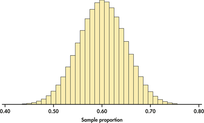

We see that both sampling distributions are centered on p=0.6. This again reflects the lack of bias in the sample proportion statistic. Notice, however, the values of ˆp for samples of size 2500 are much less spread out than for samples of size 100.
Apply Your Knowledge
Question 5.59
5.59 How much less spread?
Refer to Example 5.24 in which we showed the sampling distributions of ˆp for n=100 and n=2500 with p=0.60 in both cases.
- In terms of a multiple, how much larger is the standard deviation of the sampling distribution for n=100 versus n=2500 when p=0.60?
- Show that the multiple found in part (a) does not depend on the value of p.
5.59
(a) 5 times as large. (b) √p(1−p)100/√p(1−p)2500=√p(1−p)√100/√p(1−p)√2500=1√100/1√2500=√2500√100=5010=5
Bias and variability
The sampling distribution shown in Figure 5.13 shows that a sample of size 2500 will almost always give an estimate ˆp that is close to the truth about the population. Figure 5.13 illustrates this fact for just one value of the population proportion, but it is true for any proportion. On the other hand, as seen from Figure 5.12, samples of size 100 might give an estimate of 50% or 70% when the truth is 60%.
Thinking about Figures 5.12 and 5.13 helps us restate the idea of bias when we use a statistic like ˆp to estimate a parameter like p. It also reminds us that variability matters as much as bias.
Bias and Variability of a Statistic
Bias concerns the center of the sampling distribution. A statistic used to estimate a parameter is an unbiased estimator if the mean of its sampling distribution is equal to the true value of the parameter being estimated.
The variability of a statistic is described by the spread of its sampling distribution. This spread is determined by the sampling design and the sample size n. Statistics from larger probability samples have smaller spreads.
The margin of error is a numerical measure of the spread of a sampling distribution. It can be used to set bounds on the size of the likely error in using the statistic as an estimator of a population parameter.
The fact that the mean of ˆp is p tells us that the sample proportion ˆp in an SRS is an unbiased estimator of the population proportion p.
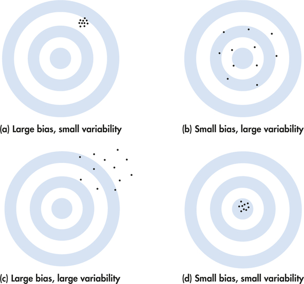
Shooting arrows at a target with a bull’s-eye is a nice way to think in general about bias and variability of any statistic, not just the sample proportion. We can think of the true value of the population parameter as the bull’s-eye on a target and of the sample statistic as an arrow fired at the bull’s-eye. Bias and variability describe what happens when an archer fires many arrows at the target. Bias means that the aim is off, and the arrows will tend to land off the bull’s-eye in the same direction. The sample values do not center about the population value. Large variability means that repeated shots are widely scattered on the target. Repeated samples do not give similar results but differ widely among themselves. Figure 5.14 shows this target illustration of the two types of error.
Notice that small variability (repeated shots are close together) can accompany large bias (the arrows are consistently away from the bull’s-eye in one direction).And small bias (the arrows center on the bull’s-eye) can accompany large variability(repeated shots are widely scattered). A good sampling scheme, like a good archer, must have both small bias and small variability. Here’s how we do this.
Managing Bias and Variability
To reduce bias, use random sampling. When we start with a list of the entire population, simple random sampling produces unbiased estimates—the values of a statistic computed from an SRS neither consistently overestimate nor consistently underestimate the value of the population parameter.
To reduce the variability of a statistic from an SRS, use a larger sample. You can make the variability as small as you want by taking a large enough sample.
In practice, the Futures Company takes only one sample. We don’t know how close to the truth an estimate from this one sample is because we don’t know what the truth about the population is. But large random samples almost always give an estimate that is close to the truth. Looking at the sampling distribution of Figure 5.13 shows that we can trust the result of one sample based on the large sample size of n=2500.
The Futures Company’s sample is fairly large and will likely provide an estimate close to the true proportion of its potential customers who have strong interest in the company’s product. Consider the monthly Current Population Survey (CPS)conducted by U.S. Bureau of Labor Statistics. In Chapter 4, we used CPS results averaged over a year in our discussions of conditional probabilities. The monthly CPS is based on a sample of 60,000 households and, as you can imagine, provides estimates of statistics such as national unemployment rate very accurately. Of course, only probability samples carry this guarantee. Using a probability sampling design and taking care to deal with practical difficulties reduce bias in a sample.

The size of the sample then determines how close to the population truth the sample result is likely to fall. Results from a sample survey usually come with a margin of error that sets bounds on the size of the likely error. The margin of error directly reflects the variability of the sample statistic, so it is smaller for larger samples. We will provide more details on margin of error in the next chapter, and it will play a critical role in subsequent chapters thereafter.
Why randomize?
Why randomize? The act of randomizing guarantees that the results of analyzing our data are subject to the laws of probability. The behavior of statistics is described by a sampling distribution. For the statistics we are most interested in, the form of the sampling distribution is known and, in many cases, is approximately Normal. Often, the center of the distribution lies at the true parameter value so that the notion that randomization eliminates bias is made more precise. The spread of the distribution describes the variability of the statistic and can be made as small as we wish by choosing a large enough sample. In a randomized experiment, we can reduce variability by choosing larger groups of subjects for each treatment.
These facts are at the heart of formal statistical inference. Chapter 6 and the following chapters have much to say in more technical language about sampling distributions and the way statistical conclusions are based on them. What any user of statistics must understand is that all the technical talk has its basis in a simple question: what would happen if the sample or the experiment were repeated many times? The reasoning applies not only to an SRS, but also to the complex sampling designs actually used by opinion polls and other national sample surveys. The same conclusions hold as well for randomized experimental designs. The details vary with the design, but the basic facts are true whenever randomization is used to produce data.

As discussed in Section 3.2 (page 137), remember that even with a well-designed sampling plan, survey samples can suffer from problems of undercoverage and nonresponse. The sampling distribution shows only how a statistic varies due to the operation of chance in randomization. It reveals nothing about possible bias due to undercoverage or nonresponse in a sample or to lack of realism in an experiment. The actual error in estimating a parameter by a statistic can be much larger than the sampling distribution suggests. What is worse, there is no way to say how large the added error is. The real world is less orderly than statistics textbooks imply.