5.1 The Binomial Distributions
 This page includes Video Technology Manuals
Counts and proportions are discrete statistics that describe categorical data. We focus our discussion on the simplest case of a random variable with only two possible categories. Here is an an example.
EXAMPLE 5.1 Cola Wars
A blind taste test of two diet colas (labeled “A” and “B”) asks 200 randomly chosen consumers which cola was preferred. We would like to view the responses of these consumers as representative of a larger population of consumers who hold similar preferences. That is, we will view the responses of the sampled consumers as an SRS from a population.
When there are only two possible outcomes for a random variable, we can summarize the results by giving the count for one of the possible outcomes. We let n represent the sample size, and we use X to represent the random variable that gives the count for the outcome of interest.
EXAMPLE 5.2 The Random Variable of Interest
In our marketing study of consumers, n=200. We will ask each consumer in our study whether he or she prefers cola A or cola B. The variable X is the number of consumers who prefer cola A. Suppose that we observe X=138.
In our example, we chose the random variable X to be the number of consumers who prefer cola A over cola B. We could have chosen X to be the number of consumers who prefer cola B over cola A. The choice is yours. Often, we make the choice based on how we would like to describe the results in a written summary.
When a random variable has only two possible outcomes, we can also use the sample proportion ˆp=X/n as a summary.
sample proportion
EXAMPLE 5.3 The Sample Proportion
The sample proportion of consumers involved in the taste test who preferred cola A is
ˆp=138200=0.67

Notice that this summary takes into account the sample size n. We need to know n in order to properly interpret the meaning of the random variable X. For example, the conclusion we would draw about consumers’ preferences would be quite different if we had observed X=138 from a sample twice as large, n=400. Be careful not to directly compare counts when the sample sizes are different. Instead, divide the counts by their associated sample sizes to allow for direct comparison.
Apply Your Knowledge

Question 5.1
5.1 Seniors who waived out of the math prerequisite.
In a random sample of 250 business students who are in or have taken business statistics, 14% reported that they had waived out of taking the math prerequisite for business statistics due to AP calculus credits from high school. Give n, X, and ˆp for this setting.
5.1
n=250, X=35, ˆp=14%.
Question 5.2
5.2 Using the Internet to make travel reservations.
A recent survey of 1351 randomly selected U.S. residents asked whether or not they had used the Internet for making travel reservations.2 There were 1041 people who answered Yes. The other 310 answered No.
- What is n?
- Choose one of the two possible outcomes to define the random variable, X. Give a reason for your choice.
- What is the value of X?
- Find the sample proportion, ˆp.
The binomial distributions for sample counts
The distribution of a count X depends on how the data are produced. Here is a simple but common situation.
The Binomial Setting
- There are a fixed number n of observations.
- The n observations are all independent. That is, knowing the result of one observation tells you nothing about the outcomes of the other observations.
- Each observation falls into one of just two categories, which, for convenience, we call “success” and “failure.”
- The probability of a success, call it p, is the same for each observation.
Think of tossing a coin n times as an example of the binomial setting. Each toss gives either heads or tails, and the outcomes of successive tosses are independent. If we call heads a success, then p is the probability of a head and remains the same as long as we toss the same coin. The number of heads we count is a random variable X. The distribution of X, and more generally the distribution of the count of successes in any binomial setting, is completely determined by the number of observations n and the success probability p.
Binomial Distribution
The distribution of the count X of successes in the binomial setting is the binomial distribution with parameters n and p. The parameter n is the number of observations, and p is the probability of a success on any one observation. The possible values of X are the whole numbers from 0 to n. As an abbreviation, we say that X is B(n, p).
The binomial distributions are an important class of discrete probability distributions. That said, the most important skill for using binomial distributions is the ability to recognize situations to which they do and don’t apply. This can be done by checking all the facets of the binomial setting.
EXAMPLE 5.4 Binomial Examples?
- Analysis of the 50 years of weekly S&P 500 price changes reveals that they are independent of each other with the probability of a positive price change being 0.56. Defining a “success” as a positive price change, let X be the number of successes over the next year, that is, over the next 52 weeks. Given the independence of trials, it is reasonable to assume that X has the B(52, 0.56) distribution.
- Engineers define reliability as the probability that an item will perform its function under specific conditions for a specific period of time. Replacement heart valves made of animal tissue, for example, have probability 0.77 of performing well for 15 years.3 The probability of failure within 15 years is, therefore, 0.23. It is reasonable to assume that valves in different patients fail (or not) independently of each other. The number of patients in a group of 500 who will need another valve replacement within 15 years has the B(500, 0.23) distribution.
- Deal 10 cards from a shuffled deck and count the number X of red cards. There are 10 observations, and each gives either a red or a black card. A “success” is a red card. But the observations are not independent. If the first card is black, the second is more likely to be red because there are more red cards than black cards left in the deck. The count X does not have a binomial distribution.
Apply Your Knowledge
In each of Exercises 5.3 to 5.6, X is a count. Does X have a binomial distribution? If so, give the distribution of X. If not, give your reasons as to why not.
Question 5.3
5.3 Toss a coin.
Toss a fair coin 20 times. Let X be the number of heads that you observe.
5.3
X~B(20,0.5)
Question 5.4
5.4 Card dealing.
Define X as the number of red cards observed in the following card dealing scenarios:
- Deal one card from a standard 52-card deck.
- Deal one card from a standard 52-card deck, record its color, return it to the deck, shuffle the cards. Repeat this experiment 10 times.
Question 5.5
5.5 Customer satisfaction calls.
The service department of an automobile dealership follows up each service encounter with a customer satisfaction survey by means of a phone call. On a given day, let X be the number of customers a service representative has to call until a customer is willing to participate in the survey.
5.5
X is not binomial; there is not a fixed number of trials n.
Question 5.6
5.6 Teaching office software.
A company uses a computer-based system to teach clerical employees new office software. After a lesson, the computer presents 10 exercises. The student solves each exercise and enters the answer. The computer gives additional instruction between exercises if the answer is wrong. The count X is the number of exercises that the student gets right.
The binomial distributions for statistical sampling
The binomial distributions are important in statistics when we wish to make inferences about the proportion p of “successes” in a population. Here is an example.

CASE 5.1 Inspecting a Supplier’s Products

A manufacturing firm purchases components for its products from suppliers. Good practice calls for suppliers to manage their production processes to ensure good quality. You can find some discussion of statistical methods for managing and improving quality in Chapter 12. There have, however, been quality lapses in the switches supplied by a regular vendor. While working with the supplier to improve its processes, the manufacturing firm temporarily institutes an acceptance sampling plan to assess the quality of shipments of switches. If a random sample from a shipment contains too many switches that don’t conform to specifications, the firm will not accept the shipment.
A quality engineer at the firm chooses an SRS of 150 switches from a shipment of 10,000 switches. Suppose that (unknown to the engineer) 8% of the switches in the shipment are nonconforming. The engineer counts the number X of nonconforming switches in the sample. Is the count X of nonconforming switches in the sample a binomial random variable?
Choosing an SRS from a population is not quite a binomial setting. Just as removing one card in Example 5.4(c) changed the makeup of the deck, removing one switch changes the proportion of nonconforming switches remaining in the shipment. If there are initially 800 nonconforming switches, the proportion remaining is 800/9999=0.080008 if the first switch drawn conforms and 799/9999=0.079908 if the first switch fails inspection. That is, the state of the second switch chosen is not independent of the first. These proportions are so close to 0.08 that, for practical purposes, we can act as if removing one switch has no effect on the proportion of nonconforming switches remaining. We act as if the count X of nonconforming switches in the sample has the binomial distribution B(150, 0.08).
Distribution of Count of Successes in an SRS
A population contains proportion p of successes. If the population is much larger than the sample, the count X of successes in an SRS of size n has approximately the binomial distribution B(n, p).
The accuracy of this approximation improves as the size of the population increases relative to the size of the sample. As a rule of thumb, we use the binomial distribution for counts when the population is at least 20 times as large as the sample.
Finding binomial probabilities
Later, we give a formula for the probability that a binomial random variable takes any of its values. In practice, you will rarely have to use this formula for calculations. Some calculators and most statistical software packages calculate binomial probabilities.
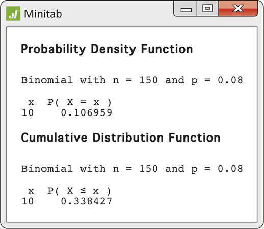
EXAMPLE 5.5 The Probability of Nonconforming Switches
CASE 5.1 The quality engineer in Case 5.1 inspects an SRS of 150 switches from a large shipment of which 8% fail to conform to specifications. What is the probability that exactly 10 switches in the sample fail inspection? What is the probability that the quality engineer finds no more than 10 nonconforming switches? Figure 5.1 shows the output from one statistical software system. You see from the output that the count X has the B(150, 0.08) distribution and
P(X=10)=0.106959P(X≤10)=0.338427
It was easy to request these calculations in the software’s menus. Typically, the output supplies more decimal places than we need and sometimes uses labels that may not be helpful (for example, “Probability Density Function” when the distribution is discrete, not continuous). But, as usual with software, we can ignore distractions and find the results we need.
If you do not have suitable computing facilities, you can still shorten the work of calculating binomial probabilities for some values of n and p by looking up probabilities in Table C in the back of this book. The entries in the table are the probabilities P(X=k) for a binomial random variable X.
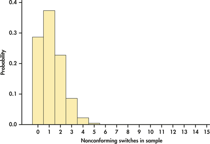
EXAMPLE 5.6 The Probability Histogram
CASE 5.1 Suppose that the quality engineer chooses just 15 switches for inspection. What is the probability that no more than one of the 15 is nonconforming? The count X of nonconforming switches in the sample has approximately the B(15, 0.08) distribution. Figure 5.2 is a probability histogram for this distribution. The distribution is strongly skewed. Although X can take any whole-number value from 0 to 15, the probabilities of values larger than 5 are so small that they do not appear in the histogram.
| p | ||
| n | k | .08 |
| 15 | 0 | .2863 |
| 1 | .3734 | |
| 2 | .2273 | |
| 3 | .0857 | |
| 4 | .0223 | |
| 5 | .0043 | |
| 6 | .0006 | |
| 7 | .0001 | |
| 8 | ||
| 9 | ||
We want to calculate
P(X≤1)=P(X=0)+P(X=1)
when X has the B(15, 0.08) distribution. To use Table C for this calculation, look opposite n=15 and under p=0.08. This part of the table appears at the left. The entry opposite each k is P(X=k). Blank entries are 0 to four decimal places, so we have omitted most of them here. From Table C,
P(X≤1)=P(X=0)+P(X=1)=0.2863+0.3734=0.6597
About two-thirds of all samples will contain no more than one nonconforming switch. In fact, almost 29% of the samples will contain no bad switches. A sample of size 15 cannot be trusted to provide adequate evidence about the presence of nonconforming items in the population. In contrast, for a sample of size 50, there is only a 1.5% risk that no bad switch will be revealed in the sample in light of the fact that 8% of the population is nonconforming. Calculations such as these can used to design acceptable acceptance sampling schemes.
The values of p that appear in Table C are all 0.5 or smaller. When the probability of a success is greater than 0.5, restate the problem in terms of the number of failures. The probability of a failure is less than 0.5 when the probability of a success exceeds 0.5. When using the table, always stop to ask whether you must count successes or failures.
EXAMPLE 5.7 Free Throws
Jessica is a basketball player who makes 75% of her free throws over the course of a season. In a key game, Jessica shoots 12 free throws and misses five of them. The fans think that she failed because she was nervous. Is it unusual for Jessica to perform this poorly?
To answer this question, assume that free throws are independent with probability 0.75 of a success on each shot. (Many studies of long sequences of basketball free throws have found essentially no evidence that they are dependent, so this is a reasonable assumption.)4 Because the probability of making a free throw is greater than 0.5, we count misses in order to use Table C. The probability of a miss is 1−0.75, or 0.25. The number X of misses in 12 attempts has the binomial distribution with n=12 and p=0.25.
We want the probability of missing five or more. This is
P(X≥5)=P(X=5)+P(X=6)+⋯+P(X=12)=0.1032+0.0401+⋯+0.0000=0.1576
Jessica will miss five or more out of 12 free throws about 16% of the time. While below her average level, her performance in this game was well within the range of the usual chance variation in her shooting.
Apply Your Knowledge
Question 5.7
5.7 Find the probabilities.
- Suppose that X has the B(7, 0.15) distribution. Use software or Table C to find P(X=0) and P(X≥5).
- Suppose that X has the B(7, 0.85) distribution. Use software or Table C to find P(X=7) and P(X≤2).
- Explain the relationship between your answers to parts (a) and (b) of this exercise.
5.7
(a) 0.3206. 0.00122 (0.0013 using Table C). (b) 0.3206. 0.00122 (0.0013 using Table C). (c) They are the same.
Question 5.8
5.8 Restaurant survey.
You operate a restaurant. You read that a sample survey by the National Restaurant Association shows that 40% of adults are committed to eating nutritious food when eating away from home. To help plan your menu, you decide to conduct a sample survey in your own area. You will use random digit dialing to contact an SRS of 20 households by telephone.
- If the national result holds in your area, it is reasonable to use the binomial distribution with n=20 and p=0.4 to describe the count X of respondents who seek nutritious food when eating out. Explain why.
- Ten of the 20 respondents say they are concerned about nutrition. Is this reason to believe that the percent in your area is higher than the national 40%? To answer this question, use software or Table C to find the probability that X is 10 or larger if p=0.4 is true. If this probability is very small, that is reason to think that p is actually greater than 0.4 in your area.
Question 5.9
5.9 Do our athletes graduate?
A university claims that at least 80% of its basketball players get degrees. To see if there is evidence to the contrary, an investigation examines the fate of 20 players who entered the program over a period of several years that ended six years ago. Of these players, 11 graduated and the remaining nine are no longer in school. If the university’s claim is true, the number of players who graduate among the 20 should have the binomial distribution with n=20 and p at least equal to 0.8.
- Use software or Table C to find the probability that 11 or less players graduate using p=0.8.
- What does the probability you found in part (a) suggest about the university’s claim?
5.9
(a) 0.01. (b) The claim is likely false.
Binomial formula
We can find a formula that generates the binomial probabilities from software or found in Table C. Finding the formula for the probability that a binomial random variable takes a particular value entails adding probabilities for the different ways of getting exactly that many successes in n observations. An example will guide us toward the formula we want.
EXAMPLE 5.8 Determining Consumer Preferences
Suppose that market research shows that your product is preferred over competitors’ products by 25% of all consumers. If X is the count of the number of consumers who prefer your product in a group of five consumers, then X has a binomial distribution with n=5 and p=0.25, provided the five consumers make choices independently. What is the probability that exactly two consumers in the group prefer your product? We are seeking P(X=2).
Because the method doesn’t depend on the specific example, we will use “S” for success and “F” for failure. Here, “S” would stand for a consumer preferring your product over the competitors’ products. We do the work in two steps.
Step 1. Find the probability that a specific two of the five consumers—say, the first and the third—give successes. This is the outcome SFSFF. Because consumers are independent, the multiplication rule for independent events applies. The probability we want is
P(SFSFF)=P(S)P(F)P(S)P(F)P(F)=(0.25)(0.75)(0.25)(0.75)(0.75)=(0.25)2(0.75)3
Step 2. Observe that the probability of any one arrangement of two S’s and three F’s has this same probability. This is true because we multiply together 0.25 twice and 0.75 three times whenever we have two S’s and three F’s. The probability that X=2 is the probability of getting two S’s and three F’s in any arrangement whatsoever. Here are all the possible arrangements:
SSFFFSFSFFSFFSFSFFFSFSSFFFSFSFFSFFSFFSSFFFSFSFFFSS
There are 10 of them, all with the same probability. The overall probability of two successes is therefore
P(X=2)=10(0.25)2(0.75)3=0.2637
Approximately 26% of the time, samples of five independent consumers will produce exactly two who prefer your product over competitors’ products.
The pattern of the calculation in Example 5.8 works for any binomial probability. To use it, we must count the number of arrangements of k successes in n observations. We use the following fact to do the counting without actually listing all the arrangements.
Binomial Coefficient
The number of ways of arranging k successes among n observations is given by the binomial coefficient
(nk)=n!k!(n−k)!
for k=0, 1, 2, …, n.
The formula for binomial coefficients uses the factorial notation. The factorial n! for any positive whole number n is
n!=n×(n−1)×(n−2)×⋯×3×2×1
factorial
Also, 0!=1. Notice that the larger of the two factorials in the denominator of a binomial coefficient will cancel much of the n! in the numerator. For example, the binomial coefficient we need for Example 5.8 is
(52)=5!2! 3!=(5)(4)(3)(2)(1)(2)(1)×(3)(2)(1)=(5)(4)(2)(1)=202=10
This agrees with our previous calculation.
The notation (nk) is not meant to represent the fraction nk. A helpful way to remember its meaning is to read it as “binomial coefficient n choose k.” Binomial coefficients have many uses in mathematics, but we are interested in them only as an aid to finding binomial probabilities. The binomial coefficient (nk) counts the number of ways in which k successes can be distributed among n observations. The binomial probability P(X=k) is this count multiplied by the probability of any specific arrangement of the k successes. Here is the formula we seek.
Binomial Probability
If X has the binomial distribution B(n, p), with n observations and probability p of success on each observation, the possible values of X are 0,1,2, . . . ,n. If k is any one of these values, the binomial probability is
P(X=k)=(nk)pk(1−p)n−k
Here is an example of the use of the binomial probability formula.
EXAMPLE 5.9 Inspecting Switches
CASE 5.1 Consider the scenario of Example 5.6 (pages 248–249) in which the number X of switches that fail inspection closely follows the binomial distribution with n=15 and p=0.08.
The probability that no more than one switch fails is
P(X≤1)=P(X=0)+P(X=1)=(150)(0.08)0(0.92)15+(151)(0.08)1(0.92)14=15!0! 15!(1)(0.2863)+15!1! 14!(0.08)(0.3112)=(1)(1)(0.2863)+(15)(0.08)(0.3112)=0.2863+0.3734=0.6597
The calculation used the facts that 0!=1 and that a0=1 for any number a≠0. The result agrees with that obtained from Table C in Example 5.6.
Apply Your Knowledge
Question 5.10
5.10 Hispanic representation.
A factory employs several thousand workers, of whom 30% are Hispanic. If the 10 members of the union executive committee were chosen from the workers at random, the number of Hispanics on the committee X would have the binomial distribution with n=10 and p=0.3.
- Use the binomial formula to find P(X=3).
- Use the binomial formula to find P(X≤3).
Question 5.11
5.11 Misleading résumés.
In Exercise 4.27 (page 190), it was stated that 18.4% of executive job applicants lied on their résumés. Suppose an executive job hunter randomly selects five résumés from an executive job applicant pool. Let X be the number of misleading résumés found in the sample.
- What are the possible values of X?
- Use the binomial formula to find the P(X=2).
- Use the binomial formula to find the probability of at least one misleading résumé in the sample.
5.11
(a) S={0, 1, 2, 3, 4, 5}. (b) 0.1840. (c) 0.6382.
Binomial mean and standard deviation
If a count X has the B(n, p) distribution, what are the mean μX and the standard deviation σX? We can guess the mean. If a basketball player makes 75% of her free throws, the mean number made in 12 tries should be 75% of 12, or 9. That’s μX when X has the B(12, 0.75) distribution.
Intuition suggests more generally that the mean of the B(n, p) distribution should be np. Can we show that this is correct and also obtain a short formula for the standard deviation? Because binomial distributions are discrete probability distributions, we could find the mean and variance by using the binomial probabilities along with general formula for computing the mean and variance given in Section 4.5. But, there is an easier way.
A binomial random variable X is the count of successes in n independent observations that each have the same probability p of success. Let the random variable Si indicate whether the ith observation is a success or failure by taking the values Si=1 if a success occurs and Si=0 if the outcome is a failure. The Si are independent because the observations are, and each Si has the same simple distribution:
| Outcome | 1 | 0 |
| Probability | p | 1−p |
From the definition of the mean of a discrete random variable, we know that the mean of each Si is
μS=(1)(p)+(0)(1−p)=p
Reminder

mean and variance of a discrete random variable, pp 235–236
Similarly, the definition of the variance shows that σ2S=p(1−p). Because each Si is 1 for a success and 0 for a failure, to find the total number of successes X we add the Si’s:
X=S1+S2+⋯+Sn
Apply the addition rules for means and variances to this sum. To find the mean of X we add the means of the Si’s:
μX=μS+μS+⋯+μS=nμS=np
Similarly, the variance is n times the variance of a single S, so that σ2X=np(1−p). The standard deviation σX is the square root of the variance. Here is the result.
Binomial Mean and Standard Deviation
If a count X has the binomial distribution B(n, p), then
μX=npσX=√np(1−p)
EXAMPLE 5.10 Inspecting Switches
CASE 5.1 Continuing Case 5.1 (page 247), the count X of nonconforming switches is binomial with n=150 and p=0.08. The mean and standard deviation of this binomial distribution are
μX=np=(150)(0.08)=12σX=√np(1−p)=√(150)(0.08)(0.92)=√11.04=3.3226
Apply Your Knowledge
Question 5.12
5.12 Hispanic representation.
Refer to the setting of Exercise 5.10 (page 253).
- What is the mean number of Hispanics on randomly chosen committees of 10 workers?
- What is the standard deviation σ of the count X of Hispanic members?
- Suppose now that 10% of the factory workers were Hispanic. Then p=0.1. What is σ in this case? What is σ if p=0.01? What does your work show about the behavior of the standard deviation of a binomial distribution as the probability of a success gets closer to 0?
Question 5.13
5.13 Do our athletes graduate?
Refer to the setting of Exercise 5.9 (page 250).
- Find the mean number of graduates out of 20 players if 80% of players graduate.
- Find the standard deviation σ of the count X if 80% of players graduate.
- Suppose now that the 20 players came from a population of which p=0.9 graduated. What is the standard deviation σ of the count of graduates? If p=0.99, what is σ? What does your work show about the behavior of the standard deviation of a binomial distribution as the probability p of success gets closer to 1?
5.13
(a) μX=16. (b) σX=1.789. (c) σX=1.342. σX=0.445. As p gets closer to 1, the standard deviation gets smaller.
Sample proportions
What proportion of a company’s sales records have an incorrect sales tax classification? What percent of adults favor stronger laws restricting firearms? In statistical sampling, we often want to estimate the proportion p of “successes” in a population. Our estimator is the sample proportion of successes:
ˆp=count of successes in samplesize of sample=Xn
proportion
Be sure to distinguish between the proportionˆp and the count X. The count takes whole-number values anywhere in the range from 0 to n, but a proportion is always a number in the range of 0 to 1. In the binomial setting, the count X has a binomial distribution. The proportion ˆp does not have a binomial distribution. We can, however, do probability calculations about ˆp by restating them in terms of the count X and using binomial methods.
EXAMPLE 5.11 Social Media Purchasing Influence
Although many companies run aggressive marketing campaigns on social media, a Gallup survey reveals that 62% of all U.S. respondents say Twitter and Facebook, among other sites, do not have any influence on their decisions to purchase products.5 It was also reported, however, that baby boomers were less likely to be influenced than younger respondents. You decide to take a nationwide random sample of 2500 college students and ask if they agree or disagree that “Social media advertising influences my purchasing decisions.” Suppose that it were the case that 45% of all college students would disagree if asked this question. In other words, 45% of all college students feel that social media has no influence on their purchasing decisions. What is the probability that the sample proportion who feel that social media has no influence is no greater than 47%?
The count X of college students who feel no influence has the binomial distribution B(2500, 0.45). The sample proportion ˆp=X/2500 does not have a binomial distribution because it is not a count. But we can translate any question about a sample proportion ˆp into a question about the count X. Because 47% of 2500 is 1175,
P(ˆp≤.047)=P(X≤1175)=P(X=0)+P(X=1)+P(X=2)+⋯+P(X=1175)
This is a rather tedious calculation. We must add 1176 binomial probabilities. Software tells us that P(ˆp≤0.47)=0.9787. But what do we do if we don’t have access to software?
As a first step in exploring the sample proportion, we need to find its mean and standard deviation. We know the mean and standard deviation of a sample count, so apply the rules from Section 4.5 for the mean and variance of a constant times a random variable. Here are the results.
Mean and Standard Deviation of a Sample Proportion
Let ˆp be the sample proportion of successes in an SRS of size n drawn from a large population having population proportion p of successes. The mean and standard deviation of ˆp are
μˆp=pσˆp=√p(1−p)n
The formula for σˆp is exactly correct in the binomial setting. It is approximately correct for an SRS from a large population. We use it when the population is at least 20 times as large as the sample.
Let’s now use these formulas to calculate the mean and standard deviation for Example 5.11.
EXAMPLE 5.12 The Mean and the Standard Deviation
The mean and standard deviation of the proportion of the college respondents in Example 5.11 who feel that social media has no influence on their purchasing decisions are
μˆp=p=0.45σˆp=√p(1−p)n=√(0.45)(0.55)2500=0.0099
In our calculations of Examples 5.11 and 5.12, we assumed that we know the proportion p of all college students who are not influenced by social media. In practical application, we, of course, do not know the true value of p. The fact that the mean of ˆp is p suggests to us that the sample proportion can serve as a reasonable estimator for the proportion of all college students. In Section 5.3, we pick up on this very discussion more formally. For now, let’s continue exploring various ways to obtain binomial-related probabilities.
Apply Your Knowledge
Question 5.14
5.14 Find the mean and the standard deviation.
If we toss a fair coin 200 times, the number of heads is a random variable that is binomial.
- Find the mean and the standard deviation of the sample proportion of heads.
- Is your answer to part (a) the same as the mean and the standard deviation of the sample count of heads? Explain your answer.
Normal approximation for counts and proportions
The binomial probability formula and tables are practical only when the number of trials n is small. Even software and statistical calculators are unable to handle calculations for very large n. Figure 5.3 shows the binomial distribution for different values of p and n. From these graphs, we see that, for a given p, the shape of the binomial distribution becomes more symmetrical as n gets larger. In particular, as the number of trials n gets larger, the binomial distribution gets closer to a Normal distribution. We can also see from Figure 5.3 that, for a given n, the binomial distribution is more symmetrical as p approaches 0.5. The upshot is that the accuracy of Normal approximation depends on the values of both n and p. Try it yourself with the Normal Approximation to Binomial Applet. This applet allows you to change n or p while watching the effect on the binomial probability histogram and the Normal curve that approximates it.
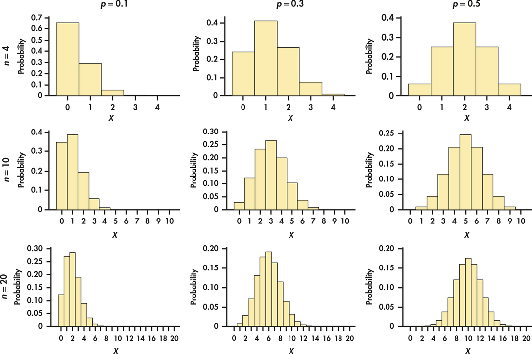

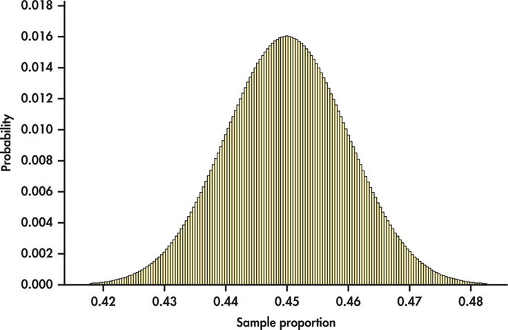
Figure 5.3 shows that the binomial count random variable X is close to Normal for large enough n. What about the sample proportion ˆp ? To clear up that matter, look at Figure 5.4. This is the probability histogram of the exact distribution of the sample proportion of college students who feel no social media influence on their purchasing decisions, based on the binomial distribution B(2500, 0.45). There are hundreds of narrow bars, one for each of the 2501 possible values of ˆp . It would be a mess to try to show all these probabilities on the graph. The key take away from the figure is that probability histogram looks very Normal!
So, with Figures 5.3 and 5.4, we have learned that both the count X and the sample proportion ˆp are approximately Normal in large samples.
Normal Approximation for Counts and Proportions
Draw an SRS of size n from a large population having population proportion p of successes. Let X be the count of successes in the sample and ˆp=X/n be the sample proportion of successes. When n is large, the distributions of these statistics are approximately Normal:
X is approximately N(np, √np(1−p))ˆp is approximately N(p, √p(1−p)n)
As a rule of thumb, we use this approximation for values of n and p that satisfy np≥10 and n(1−p)≥10
These Normal approximations are easy to remember because they say that ˆp and X are Normal, with their usual means and standard deviations. Whether or not you use the Normal approximations should depend on how accurate your calculations need to be. For most statistical purposes, great accuracy is not required. Our “rule of thumb” for use of the Normal approximations reflects this judgment.
EXAMPLE 5.13 Compare the Normal Approximation with the Exact Calculation
Let’s compare the Normal approximation for the calculation of Example 5.11 (page 255) with the exact calculation from software. We want to calculate P(ˆp≤0.47) when the sample size is n=2500 and the population proportion is p=0.45. Example 5.12 (page 256) shows that
μˆp=p=0.45σˆp=√p(1−p)n=0.0099
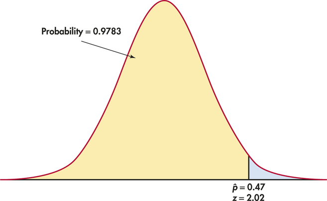
Act as if ˆp were Normal with mean 0.45 and standard deviation 0.0099. The approximate probability, as illustrated in Figure 5.5, is
P(ˆp≤0.47)=P(ˆp−0.450.0099≤0.47−0.450.0099)=P(Z≤2.02)=0.9783
That is, about 98% of all samples have a sample proportion that is at most 0.47. Because the sample was large, this Normal approximation is quite accurate. It misses the software value 0.9787 by only 0.0004.
EXAMPLE 5.14 Using the Normal Approximation
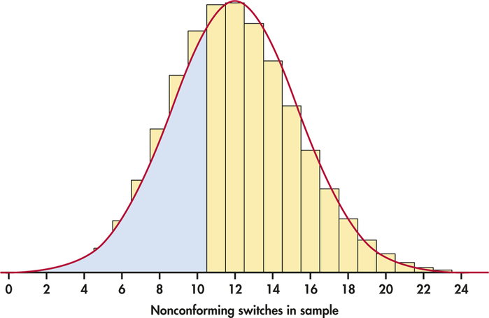
CASE 5.1 As described in Case 5.1 (page 247), a quality engineer inspects an SRS of 150 switches from a large shipment of which 8% fail to meet specifications. The count X of nonconforming switches in the sample were thus assumed to be the B(150, 0.08) distribution. In Example 5.10 (page 254), we found μX=12 and σX=3.3226.
The Normal approximation for the probability of no more than 10 nonconforming switches is the area to the left of X=10 under the Normal curve. Using Table A,
P(X≤10)=P(X−123.3226≤10−123.3226)=P(Z≤−0.60)=0.2743
In Example 5.5 (pages 247–248), we found that software tells us that the actual binomial probability that there is no more than 10 nonconforming switches in the sample is P(X≤10)=0.3384. The Normal approximation is only roughly accurate. Because np=12, this combination of n and p is close to the border of the values for which we are willing to use the approximation.
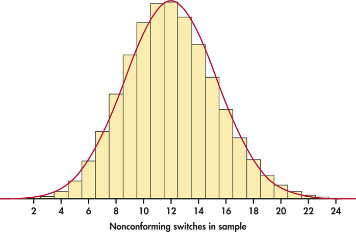
The distribution of the count of nonconforming switches in a sample of 15 is distinctly non-Normal, as Figure 5.2 (page 249) showed. When we increase the sample size to 150, however, the shape of the binomial distribution becomes roughly Normal. Figure 5.6 displays the probability histogram of the binomial distribution with the density curve of the approximating Normal distribution superimposed. Both distributions have the same mean and standard deviation, and for both the area under the histogram and the area under the curve are 1. The Normal curve fits the histogram reasonably well. But, look closer: the histogram is slightly skewed to the right, a property that the symmetric Normal curve can’t quite match.
Apply Your Knowledge
Question 5.15
5.15 Use the Normal approximation.
Suppose that we toss a fair coin 200 times. Use the Normal approximation to find the probability that the sample proportion of heads is
- between 0.4 and 0.6.
- between 0.45 and 0.55.
5.15
(a) 0.9954. (b) 0.8414.
Question 5.16
5.16 Restaurant survey.
Return to the survey described in Exercise 5.8 (page 250). You plan to use random digit dialing to contact an SRS of 200 households by telephone rather than just 20.
- What are the mean and standard deviation of the number of nutrition conscious people in your sample if p=0.4 is true?
- What is the probability that X lies between 75 and 85? (Use the Normal approximation.)
Question 5.17
5.17 The effect of sample size.
The SRS of size 200 described in the previous exercise finds that 100 of the 200 respondents are concerned about nutrition. We wonder if this is reason to conclude that the percent in your area is higher than the national 40%.
- Find the probability that X is 100 or larger if p=0.4 is true. If this probability is very small, that is reason to think that p is actually greater than 0.4 in your area.
- In Exercise 5.8, you found P(X≥10) for a sample of size 20. In part (a), you have found P(X≥100) for a sample of size 200 from the same population. Both of these probabilities answer the question, “How likely is a sample with at least 50% successes when the population has 40% successes?” What does comparing these probabilities suggest about the importance of sample size?
5.17
(a) 0.0019. (b) The larger sample gives a much smaller probability, suggesting a greater ability to detect differences.
The continuity correction
Figure 5.7 illustrates an idea that greatly improves the accuracy of the Normal approximation to binomial probabilities. The binomial probability P(X≤10) is the area of the histogram bars for values 0 to 10. The bar for X=10 actually extends from 9.5 to 10.5. Because the discrete binomial distribution puts probability only on whole numbers, the probabilities P(X≤10) and P(X≤10.5) are the same. The Normal distribution spreads probability continuously, so these two Normal probabilities are different. The Normal approximation is more accurate if we consider X=10 to extend from 9.5 to 10.5, matching the bar in the probability histogram.
The event {X≤10} includes the outcome X=10. Figure 5.7 shades the area under the Normal curve that matches all the histogram bars for outcomes 0 to 10, bounded on the right not by 10, but by 10.5. So P(X≤10) is calculated as P(X≤10.5). On the other hand, P(X<10) excludes the outcome X=10, so we exclude the entire interval from 9.5 to 10.5 and calculate P(X≤9.5) from the Normal table. Here is the result of the Normal calculation in Example 5.14 improved in this way:
P(X≤10)=P(X≤10.5)=P(X−123.3226≤10.5−123.3226)=P(Z≤−0.45)=0.3264
The improved approximation misses the exact binomial probability value of 0.3384 by only 0.012. Acting as though a whole number occupies the interval from 0.5 below to 0.5 above the number is called the continuity correction to the Normal approximation. If you need accurate values for binomial probabilities, try to use software to do exact calculations. If no software is available, use the continuity correction unless n is very large. Because most statistical purposes do not require extremely accurate probability calculations, the use of the continuity correction can be viewed as optional.
continuity correction
Assessing binomial assumption with data
In the examples of this section, the probability calculations rest on the assumption that the count random variable X is well described by the binomial distribution. Our confidence with such an assumption depends to a certain extent on the strength of our belief that the conditions of the binomial setting are at play. But ultimately we should allow the data to judge the validity of our beliefs. In Chapter 1, we used the Normal quantile data tool to check the compatibility of the data with the unique features of the Normal distribution. The binomial distribution has its own unique features that we can check as to whether or not they are reflected in the data. Let’s explore the applicability of the binomial distribution with the following example.
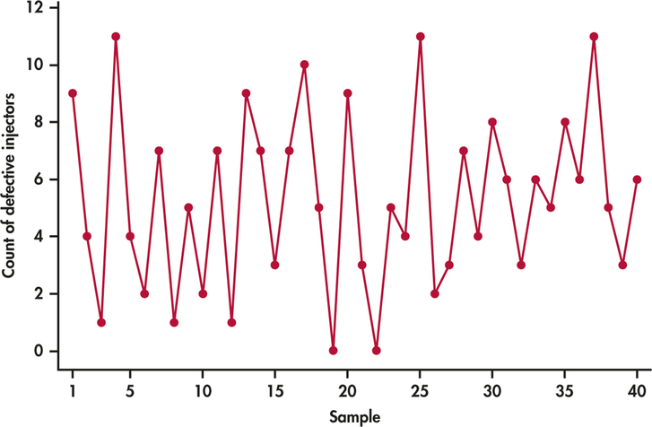
EXAMPLE 5.15 Checking for Binomial Compatibility
inject
Consider an application in which n=200 manufactured fuel injectors are sampled periodically to check for compliance to specifications. Figure 5.8 shows the counts of defective injectors found in 40 consecutive samples. The counts appear to be behaving randomly over time. Summing over the 40 samples, we find the total number of observed defects to be 210 out of the 8000 total number of injectors inspected. This is associated with a proportion defective of 0.02625. Assuming that the random variable X of the defect counts for each sample follows the B(200, 0.02625), the standard deviation of X will have a value around
σˆp=√np(1−p)=√200(0.02625)(0.97375)=2.26
In terms of variance, the variance of the counts is expected to be around 2.262 or 5.11. Computing the sample variance s2 on the observed counts, we would find a variance of 9.47. The observed variance of the counts is nearly twice of what is expected if the counts were truly following the binomial distribution. It appears that the binomial model does not fully account for the overall variation of the counts.
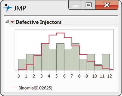
The statistical software JMP provides a nice option of superimposing a binomial distribution fit on the observed counts. Figure 5.9 shows the B(200, 0.02625) distribution overlaid on the histogram of the count data. The mismatch between the binomial distribution fit and the observed counts is clear. The observed counts are spread out more than expected by the binomial distribution, with a greater number of counts found both at the lower and upper ends of the histogram.
The defect count data of Example 5.15 are showing overdispersion in that the counts have greater variability than expected from the assumed count distribution. Likely explanations for the extra variability are changes in the probability of defects between production runs due to adjustments in machinery, changes in the quality of incoming raw material, and even changes in personnel. As it currently stands, it would be ill advised to base probability computations for the defect process on the binomial distribution.
Overdispersion