8 Inference for Proportions

8.2 Comparing Two Proportions

This page includes Video Technology Manuals

This page includes Statistical Videos

Because comparative studies are so common, we often want to compare the proportions of two groups (such as men and women) that have some characteristic. We call the two groups being compared Population 1 and Population 2 and the two population proportions of “successes” $p_{1}$ and $p_{2}$ . The data consist of two independent SRSs. The sample sizes are $n_{1}$ for Population 1 and $n_{2}$ for Population 2. The proportion of successes in each sample estimates the corresponding population proportion. Here is the notation we will use in this section:

Population	Population proportion	Sample size	Count of successes	Sample proportion
1	$p_{1}$	$n_{1}$	$X_{1}$	${\hat{p}}_{1} = X_{1} / n_{1}$
2	$p_{2}$	$n_{2}$	$X_{2}$	${\hat{p}}_{2} = X_{2} / n_{2}$

To compare the two unknown population proportions, start with the observed difference between the two sample proportions,

$D = {\hat{p}}_{1} - {\hat{p}}_{2}$

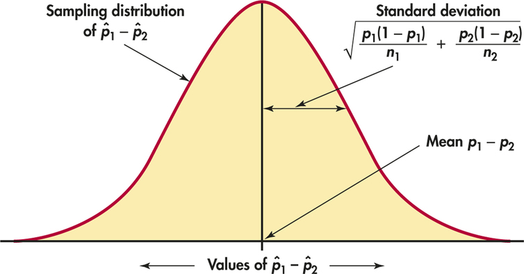
When both sample sizes are sufficiently large, the sampling distribution of the difference $D$ is approximately Normal. What are the mean and the standard deviation of $D$ ? Each of the two $\hat{p}$ 's has the mean and standard deviation given in the box on pages 418–419. Because the two samples are independent, the two $\hat{p}$ 's are also independent. We can apply the rules for means and variances of sums of random variables. Here is the result, which is summarized in Figure 8.5.

Sampling Distribution of ${\hat{p}}_{1} - {\hat{p}}_{2}$

Choose independent SRSs of sizes $n_{1}$ and $n_{2}$ from two populations with proportions $p_{1}$ and $p_{2}$ of successes. Let $D = {\hat{p}}_{1} - {\hat{p}}_{2}$ be the difference between the two sample proportions of successes. Then

As both sample sizes increase, the sampling distribution of $D$ becomes approximately Normal.
The mean of the sampling distribution is $p_{1} - p_{2}$ .
The standard deviation of the sampling distribution is
$σ_{D} = \sqrt{\frac{p_{1} (1 - p_{1})}{n_{1}} + \frac{p_{2} (1 - p_{2})}{n_{2}}}$

FIGURE 8.5 The sampling distribution of the difference between two sample proportions is approximately Normal. The mean and standard deviation are found from the two population proportions of successes,

$p_{1}$ and

$p_{2}$ .

Page 437

Apply Your Knowledge

Question 8.49

8.49 Rules for means and variances.

Suppose $p_{1} = 0.3$ , $n_{1} = 35$ , $p_{2} = 0.5$ , and $n_{2} = 30$ . Find the mean and the standard deviation of the sampling distribution of ${\hat{p}}_{1} - {\hat{p}}_{2}$ .

8.49

$μ_{{\hat{p}}_{1} - {\hat{p}}_{2}} = - 0.2, σ_{{\hat{p}}_{1} - {\hat{p}}_{2}} = 0.12$ .

Question 8.50

8.50 Effect of the sample sizes.

Suppose $p_{1} = 0.3$ , $n_{1} = 140$ , $p_{2} = 0.5$ , and $n_{2} = 120$ .

Find the mean and the standard deviation of the sampling distribution of ${\hat{p}}_{1} - {\hat{p}}_{2}$ .
The sample sizes here are four times as large as those in the previous exercise, while the population proportions are the same. Compare the results for this exercise with those that you found in the previous exercise. What is the effect of multiplying the sample sizes by 4?

Question 8.51

8.51 Rules for means and variances.

It is quite easy to verify the mean and standard deviation of the difference $D$ .

What are the means and standard deviations of the two sample proportions ${\hat{p}}_{1}$ and ${\hat{p}}_{2}$ ? (Look at the box on page 256 if you need to review this.)
Use the addition rule for means of random variables: what is the mean of $D = {\hat{p}}_{1} - {\hat{p}}_{2}$ ?
The two samples are independent. Use the addition rule for variances of random variables to find the variance of $D$ .

8.51

(a) $\begin{array}{l} μ_{{\hat{p}}_{1}} = p_{1}, σ_{{\hat{p}}_{1}} = \sqrt{\frac{p_{1} (1 - p_{1})}{n_{1}}} . \\ μ_{{\hat{p}}_{2}} = p_{2}, σ_{{\hat{p}}_{2}} = \sqrt{\frac{p_{2} (1 - p_{2})}{n_{2}}} . \end{array}$

(b) $μ_{{\hat{p}}_{1} - {\hat{p}}_{2}} = μ_{{\hat{p}}_{1}} - μ_{{\hat{p}}_{2}} = p_{1} - p_{2} .$

(c) $σ_{{\hat{p}}_{1} - {\hat{p}}_{2}}^{2} = σ_{{\hat{p}}_{1}}^{2} + {(- 1)}^{2} σ_{{\hat{p}}_{2}}^{2} = \frac{p_{1} (1 - p_{1})}{n_{1}} + \frac{p_{2} (1 - p_{2})}{n_{2}} .$

Large-sample confidence intervals for a difference in proportions

The large-sample estimate of the difference in two proportions $p_{1} - p_{2}$ is the corresponding difference in sample proportions ${\hat{p}}_{1} - {\hat{p}}_{2}$ . To obtain a confidence interval for the difference, we once again replace the unknown parameters in the standard deviation by estimates to obtain an estimated standard deviation, or standard error. Here is the confidence interval we want.

Confidence Interval for Comparing Two Proportions

Choose an SRS of size $n_{1}$ from a large population having proportion $p_{1}$ of successes and an independent SRS of size $n_{2}$ from another population having proportion $p_{2}$ of successes.

The large-sample estimate of the difference in proportions is

$D = {\hat{p}}_{1} - {\hat{p}}_{2} = \frac{X_{1}}{n_{1}} - \frac{X_{2}}{n_{2}}$

The standard error of the difference is

${SE}_{D} = \sqrt{\frac{{\hat{p}}_{1} (1 - {\hat{p}}_{1})}{n_{1}} + \frac{{\hat{p}}_{2} (1 - {\hat{p}}_{2})}{n_{2}}}$

and the margin of error for confidence level C is

$m = z^{*} {SE}_{D}$

where $z^{*}$ is the value for the standard Normal density curve with area C between $- z^{*}$ and $z^{*}$ . The large-sample level C confidence interval for $p_{1} - p_{2}$ is

$({\hat{p}}_{1} - {\hat{p}}_{2}) \pm m$

Use this method when the number of successes and the number of failures in each of the samples are at least 10.

Page 438

CASE 8.3 Social Media in the Supply Chain

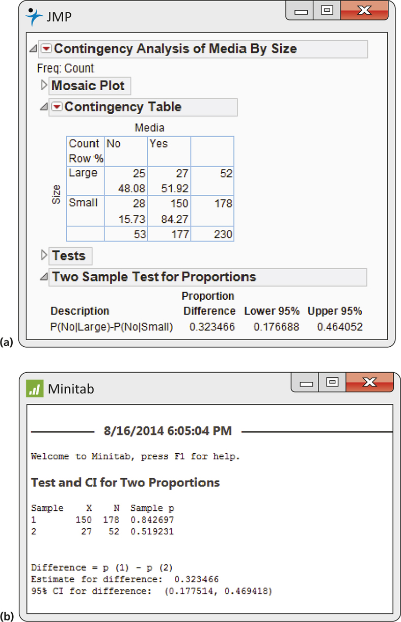
In addition to traditional marketing strategies, marketing through social media has assumed an increasingly important component of the supply chain. This is particularly true for relatively small companies that do not have large marketing budgets. One study of Austrian food and beverage companies compared the use of audio/video sharing through social media by large and small companies.¹³ Companies were classified as small or large based on whether their annual sales were greater than or less than 135 million euros. We use company size as the explanatory variable. It is categorical with two possible values. Media is the response variable with values Yes for the companies who use audio/visual sharing on social media in their supply chain, and No if they do not.

Here is a summary of the data. We let $X$ denote the count of the number of companies that use audio/visual sharing.

Size	$n$	$X$	$\hat{p} = X / n$
1 (small companies)	178	150	0.8427
2 (large companies)	52	27	0.5192

The study in Case 8.3 suggests that smaller companies are more likely to use audio/visual sharing through social media than are large companies. Let's explore this possibility using a confidence interval.

EXAMPLE 8.8 Small Companies versus Large Companies

CASE 8.3 First, we find the estimate of the difference:

$D = {\hat{p}}_{1} - {\hat{p}}_{2} = \frac{X_{1}}{n_{1}} - \frac{X_{2}}{n_{2}} = 0.8427 - 0.5192 = 0.3235$

Next, we calculate the standard error:

${SE}_{D} = \sqrt{\frac{0.8427 (1 - 0.8427)}{178} + \frac{0.5192 (1 - 0.5192)}{52}} = 0.07447$

For 95% confidence, we use $z^{*} = 1.96$ , so the margin of error is

$m = z^{*} {SE}_{D} = (1.96) (0.07447) = 0.1460$

The large-sample 95% confidence interval is

$D \pm m = 0.3235 \pm 0.1460 = (0.18, 0.47)$

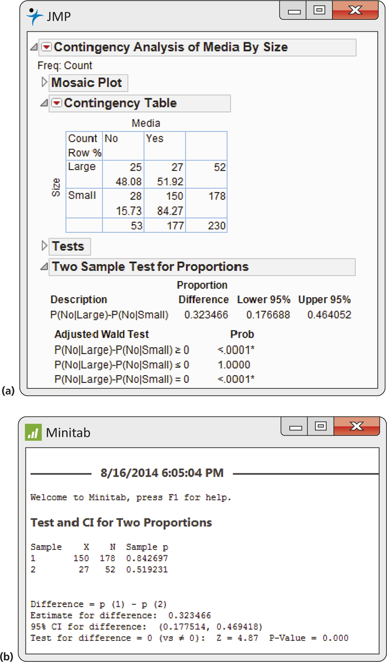
With 95% confidence, we can say that the difference in the proportions is between 0.18 and 0.47. Alternatively, we can report that the percent usage of audio/ visual sharing through social media by smaller companies is about 32% higher than the percent for large companies, with a 95% margin of error of 15%.

JMP and Minitab for Example 8.8 appear in Figure 8.6. Note that JMP uses a different approximation than the one that we studied and that is used by Minitab. Other statistical packages provide output that is similar.

In surveys such as this, small companies and large companies typically are not sampled separately. The respondents to a single sample of companies are classified after the fact as small or large. The sample sizes are then random and reflect the characteristics of the population sampled. Two-sample significance tests and confidence intervals are still approximately correct in this situation, even though the two sample sizes were not fixed in advance.

Page 439

FIGURE 8.6 JMP and Minitab outputs, Example 8.8: (a) JMP; (b) Minitab.

In Example 8.8, we chose small companies to be the first population. Had we chosen large companies as the first population, the estimate of the difference would be negative (−0.3235). Because it is easier to discuss positive numbers, we generally choose the first population to be the one with the higher proportion. The choice does not affect the substance of the analysis. It does make it easier to communicate the results.

Apply Your Knowledge

Question 8.52

8.52 Gender and commercial preference.

A study was designed to compare two energy drink commercials. Each participant was shown the commercials in random order and was asked to select the better one. Commercial A was selected by 44 out of 100 women and 79 out of 140 men. Give an estimate of the difference in gender proportions that favored Commercial A. Also construct a large-sample 95% confidence interval for this difference.

Page 440

Question 8.53

8.53 Gender and commercial preference, revisited.

Refer to Exercise 8.52. Construct a 95% confidence interval for the difference in proportions that favor Commercial B. Explain how you could have obtained these results from the calculations you did in Exercise 8.52.

8.53

(−0.003, 0.252). We can just reverse the sign of the interval in the previous exercise.

Plus four confidence intervals for a difference in proportions

Just as in the case of estimating a single proportion, a small modification of the sample proportions greatly improves the confidence intervals.¹⁴ The confidence intervals will be approximately the same as the $z$ confidence intervals when the criteria using those intervals are satisfied. When the criteria are not met, the plus four intervals will still be valid when both sample sizes are at least five and the confidence level is 90%, 95%, or 99%.

As before, we first add two successes and two failures to the actual data, dividing them equally between the two samples. That is, add one success and one failure to each sample. Note that we have added 2 to $n_{1}$ and to $n_{2}$ . We then perform the calculations for the $z$ procedure with the modified data. As in the case of a single sample, we use the term Wilson estimates for the estimates produced in this way.

Wilson estimates

In Example 8.8, we had $X_{1} = 150, n_{1} = 178, X_{2} = 27$ , and $n_{2} = 52$ . For the plus four procedure, we would use $X_{1} = 151, n_{1} = 180, X_{2} = 28$ , and $n_{2} = 54$ .

Apply Your Knowledge

Question 8.54

8.54 Social media and the supply chain using plus four.

Refer to Example 8.8 (page 438), where we computed a 95% confidence interval for the difference in the proportions of small companies and large companies that use audio/visual sharing through social media as part of their supply chain. Redo the computations using the plus four method, and compare your results with those obtained in Example 8.8.

Question 8.55

8.55 Social media and the supply chain using plus four.

Refer to the previous exercise and to Example 8.8. Suppose that the sample sizes were smaller but that the proportions remained approximately the same. Specifically, assume that 17 out of 20 small companies used social media and 13 out of 25 large companies used social media. Compute the plus four interval for 95% confidence. Then, compute the corresponding $z$ interval and compare the results.

8.55

The plus-four interval is (0.052, 0.548). The $z$ interval is (0.079, 0.581). The intervals are somewhat different when the sample sizes are small.

Question 8.56

8.56 Gender and commercial preference.

Refer to Exercises 8.52 and 8.53, where you analyzed data about gender and the preference for one of two commercials. The study also asked the same subjects to give a preference for two other commercials, C and D. Suppose that 92 women preferred Commercial C and that 120 men preferred Commercial C.

The $z$ confidence interval for comparing two proportions should not be used for these data. Why?
Compute the plus four confidence interval for the difference in proportions.

Significance tests

Although we prefer to compare two proportions by giving a confidence interval for the difference between the two population proportions, it is sometimes useful to test the null hypothesis that the two population proportions are the same.

Page 441

We standardize $D = {\hat{p}}_{1} - {\hat{p}}_{2}$ by subtracting its mean $p_{1} - p_{2}$ and then dividing by its standard deviation

$σ_{D} = \sqrt{\frac{p_{1} (1 - p_{1})}{n_{1}} + \frac{p_{2} (1 - p_{2})}{n_{2}}}$

If $n_{1}$ and $n_{2}$ are large, the standardized difference is approximately $N (0, 1)$ . To get a confidence interval, we used sample estimates in place of the unknown population proportions $p_{1}$ and $p_{2}$ in the expression for $σ_{D}$ . Although this approach would lead to a valid significance test, we follow the more common practice of replacing the unknown $σ_{D}$ with an estimate that takes into account the null hypothesis that $p_{1} = p_{2}$ . If these two proportions are equal, we can view all the data as coming from a single population. Let $p$ denote the common value of $p_{1}$ and $p_{2}$ . The standard deviation of $D = {\hat{p}}_{1} - {\hat{p}}_{2}$ is then

$\begin{array}{l} σ_{D p} & = & \sqrt{\frac{p (1 - p)}{n_{1}} + \frac{p (1 - p)}{n_{2}}} \\ = & \sqrt{p (1 - p) (\frac{1}{n_{1}} + \frac{1}{n_{2}})} \end{array}$

The subscript on $σ_{D p}$ reminds us that this is the standard deviation under the special condition that the two populations share a common proportion $p$ of successes.

We estimate the common value of $p$ by the overall proportion of successes in the two samples:

$\hat{p} = \frac{number of successes in both samples}{number of observations in both samples} = \frac{X_{1} + X_{2}}{n_{1} + n_{2}}$

This estimate of $p$ is called the pooled estimate because it combines, or pools, the information from two independent samples.

pooled estimate of $p$

To estimate the standard deviation of $D$ , substitute $\hat{p}$ for $p$ in the expression for $σ_{D p}$ . The result is a standard error for $D$ under the condition that the null hypothesis $H_{0} : p_{1} = p_{2}$ is true. The test statistic uses this standard error to standardize the difference between the two sample proportions.

Significance Tests for Comparing Two Proportions

Choose an SRS of size $n_{1}$ from a large population having proportion $p_{1}$ of successes and an independent SRS of size $n_{2}$ from another population having proportion $p_{2}$ of successes. To test the hypothesis

$H_{0} : p_{1} = p_{2}$

compute the $z$ statistic

$z = \frac{{\hat{p}}_{1} - {\hat{p}}_{2}}{{SE}_{D p}}$

where the pooled standard error is

${SE}_{D p} = \sqrt{\hat{p} (1 - \hat{p}) (\frac{1}{n_{1}} + \frac{1}{n_{2}})}$

based on the pooled estimate of the common proportion of successes

$\hat{p} = \frac{X_{1} + X_{2}}{n_{1} + n_{2}}$

Page 442

In terms of a standard Normal random variable $Z$ , the $P$ -value for a test of $H_{0}$ against

$\begin{array}{l} H_{a} : p_{1} > p_{2} & is & P (Z \geq z) \end{array}$

$\begin{array}{l} H_{a} : p_{1} < p_{2} & is & P (Z \leq z) \end{array}$

$\begin{array}{l} H_{a} : p_{1} \neq p_{2} & is & 2 P (Z \geq | z |) \end{array}$

Use this test when the number of successes and the number of failures in each of the samples are at least five.

EXAMPLE 8.9 Social Media in the Supply Chain

CASE 8.3 Example 8.8 (page 438) analyzes data on the use of audio/visual sharing through social media by small and large companies. Are the proportions of social media users the same for the two types of companies? Here is the data summary:

Size	$n$	$X$	$\hat{p} = X / n$
1 (small companies)	178	150	0.8427
2 (large companies)	52	27	0.5192

The sample proportions are certainly quite different, but we need a significance test to verify that the difference is too large to easily result from the role of chance in choosing the sample. Formally, we compare the proportions of social media users in the two populations (small companies and large companies) by testing the hypotheses

$\begin{array}{l} H_{0} : p_{1} = p_{2} \\ H_{a} : p_{1} \neq p_{2} \end{array}$

The pooled estimate of the common value of $p$ is

$\hat{p} = \frac{150 + 27}{178 + 52} = \frac{177}{230} = 0.7696$

This is just the proportion of label users in the entire sample.

First, we compute the standard error

${SE}_{D p} = \sqrt{(0.7696) (1 - 0.7696) (\frac{1}{178} + \frac{1}{52})} = 0.0664$

and then we use this in the calculation of the test statistic

$z = \frac{{\hat{p}}_{1} - {\hat{p}}_{2}}{{SE}_{D p}} = \frac{0.8427 - 0.5192}{0.0664} = 4.87$

The difference in the sample proportions is almost five standard deviations away from zero. The $P$ -value is $2 P (Z \geq 4.87)$ . In Table A, the largest entry we have is $z = 3.49$ with $P (Z \leq 3.49) = 0.9998$ . So, $P (Z > 3.49) = 1 - 0.9998 = 0.0002$ . Therefore, we can conclude that $P < 2 \times 0.0002 = 0.0004$ . Our report: 84% of small companies use audio/visual sharing through social media versus 52% of large companies; the difference is statistically significant $z = 4.87, P < 0.0004$ .

Page 443

Figure 8.7 gives the JMP and Minitab outputs for Example 8.9. Carefully examine the output to find all the important pieces that you would need to report the results of the analysis and to draw a conclusion. Note that the slight differences in results is due to the use of different approximations.

Some experts would expect the usage of social media would be greater for small companies than for large companies because small companies do not have the resources for large expensive marketing efforts. These experts might choose the one-sided alternative $H_{a} : p_{1} > p_{2}$ . The $P$ -value would be half of the value obtained for the two-sided test. Because the $z$ statistic is so large, this distinction is of no practical importance.

FIGURE 8.7 JMP and Minitab outputs, Example 8.9: (a) JMP; (b) Minitab.

Page 444

Apply Your Knowledge

Question 8.57

8.57 Gender and commercial preference

Refer to Exercise 8.52 (page 439), which compared women and men with regard to their preference for one of two commercials.

State appropriate null and alternative hypotheses for this setting. Give a justification for your choice.
Use the data given in Exercise 8.52 (page 439) to perform a two-sided significance test. Give the test statistic and the $P$ -value.
Summarize the results of your significance test.

8.57

(a) $H_{0} : p_{1} = p_{2}, H_{a} : p_{1} \neq p_{2}$ . Not knowing anything about the two commercials, there is no reason to believe men or women will prefer Commercial A more, so the test should be two-sided. (b) $Z = - 1.90, P -value = 0.0574$ . (c) The data do not show evidence of a difference between women and men concerning preference of Commercial A.

Question 8.58

8.58 What about preference for Commercial B

Refer to Exercise 8.53 (page 440), where we changed the roles of the two commercials in our analysis. Answer the questions given in the previous exercise for the data altered in this way. Describe the results of the change.

Choosing a sample size for two sample proportions

In Section 8.1, we studied methods for determining the sample size using two settings. First, we used the margin of error for a confidence interval for a single proportion as the criterion for choosing $n$ (page 427). Second, we used the power of the significance test for a single proportion as the determining factor (page 429). We follow the same approach here for comparing two proportions.

Use the margin of error

Recall that the large-sample estimate of the difference in proportions is

$D = {\hat{p}}_{1} - {\hat{p}}_{2} = \frac{X_{1}}{n_{1}} - \frac{X_{2}}{n_{2}}$

the standard error of the difference is

${SE}_{D} = \sqrt{\frac{{\hat{p}}_{1} (1 - {\hat{p}}_{1})}{n_{1}} + \frac{{\hat{p}}_{2} (1 - {\hat{p}}_{2})}{n_{2}}}$

and the margin of error for confidence level C is

$m = z^{*} {SE}_{D}$

where $z^{*}$ is the value for the standard Normal density curve with area C between $- z^{*}$ and $z^{*}$ .

For a single proportion, we picked guesses for the true proportion and computed the margins of error for various choices of $n$ . We can display the results in a table, as in Example 8.6 (page 428), or in a graph, as in Exercise 8.45 (page 435).

Sample Size for Desired Margin of Error

The level C confidence interval for a difference in two proportions will have a margin of error approximately equal to a specified value $m$ when the sample size for each of the two proportions is

$n = {(\frac{z^{*}}{m})}^{2} (p_{1}^{*} (1 - p_{1}^{*}) + p_{2}^{*} (1 - p_{2}^{*}))$

Here $z^{*}$ is the critical value for confidence C, and $p_{1}^{*}$ and $p_{2}^{*}$ are guessed values for $p_{1}$ and $p_{2}$ , the proportions of successes in the future sample.

Page 445

The margin of error will be less than or equal to $m$ if $p_{1}^{*}$ and $p_{2}^{*}$ are chosen to be 0.5. The common sample size required is then given by

$n = (\frac{1}{2}) {(\frac{z^{*}}{m})}^{2}$

Note that to use the confidence interval that is based on the Normal approximation, we still require that the number of successes and the number of failures in each of the samples are at least 10.

EXAMPLE 8.10 Confidence Interval-Based Sample Sizes for Preferences of Women and Men

Consider the setting in Exercise 8.52 (page 439), where we compared the preferences of women and men for two commercials. Suppose we want to do a study in which we perform a similar comparison using a 95% confidence interval that will have a margin of error of 0.1 or less. What should we choose for our sample size? Using $m = 0.1$ and $z^{*}$ in our formula, we have

$n = (\frac{1}{2}) {(\frac{z^{*}}{m})}^{2} = (\frac{1}{2}) {(\frac{1.96}{0.1})}^{2} = 192.08$

We would include 192 women and 192 men in our study.

Note that we have rounded the calculated value, 192.08, down because it is very close to 192. The normal procedure would be to round the calculated value up to the next larger integer.

Apply Your Knowledge

Question 8.59

8.59 What would the margin of error be?

Consider the setting in Example 8.10.

Compute the margins of error for $n_{1} = 24$ and $n_{2} = 24$ for each of the following scenarios: $p_{1} = 0.6$ , $p_{2} = 0.5$ ; $p_{1} = 0.7$ , $p_{2} = 0.5$ ; and $p_{1} = 0.8$ , $p_{2} = 0.5$ .
If you think that any of these scenarios is likely to fit your study, should you reconsider your choice of $n_{1} = 24$ and $n_{2} = 24$ ? Explain your answer.

8.59

(a) 0.28. 0.27. 0.26. (b) Yes, under all three conditions, the margin of error is much larger than the desired 0.1 as given in Example 8.10.

Use the power of the significance test

When we studied using power to compute the sample size needed for a significance test for a single proportion, we used software. We will do the same for the significance test for comparing two proportions.

Some software allows us to consider significance tests that are a little more general than the version we studied in this section. Specifically, we used the null hypothesis $H_{0} : p_{1} = p_{2}$ , which we can rewrite as $H_{0} : p_{1} - p_{2} = 0$ . The generalization allows us to use values different from zero in the alternative way of writing $H_{0}$ . Therefore, we write $H_{0} : p_{1} - p_{2} = Δ_{0}$ for the null hypothesis, and we will need to specify $Δ_{0} = 0$ for the significance test that we studied.

Here is a summary of the inputs needed for software to perform the calculations:

the value of $Δ_{0}$ in the null hypothesis $H_{0} : p_{1} - p_{2} = Δ_{0}$
the alternative hypothesis, two-sided ( $H_{a} : p_{1} \neq p_{2}$ ) or one-sided ( $H_{a} : p_{1} > p_{2}$ or $H_{a} : p_{1} < p_{2}$ )
values for $p_{1}$ and $p_{2}$ in the alternative hypothesis
Page 446
the type I error ( $α$ , the probability of rejecting the null hypothesis when it is true); usually we choose 5% ( $α = 0.05$ ) for the type I error
power (probability of rejecting the null hypothesis when it is false); usually we choose 80% (0.80) for power

EXAMPLE 8.11 Sample Sizes for Preferences of Women and Men

Refer to Example 8.10, where we used the margin of error to find the sample sizes for comparing the preferences of women and men for two commercials. Let's find the sample sizes required for a significance test that the two proportions who prefer Commercial A are equal ( $Δ_{0} = 0$ ) using a two-sided alternative with $p_{1} = 0.6$ and $p_{2} = 0.4$ , $α = 0.05$ , and 80% (0.80) power. Outputs from JMP and Minitab are given in Figure 8.8. We need $n_{1} = 97$ women and $n_{2} = 97$ men for our study.

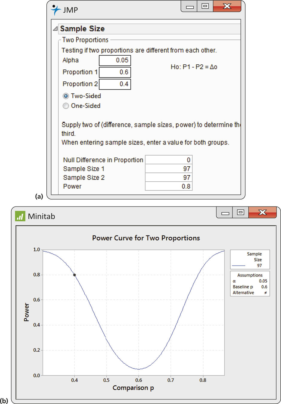
FIGURE 8.8 JMP and Minitab outputs, Example 8.11: (a) JMP; (b) Minitab.

Page 447

Note that the Minitab output (Figure 8.8(b)) gives the power curve for different alternatives. All of these have $p_{1} = 0.6$ , which Minitab calls the “Comparison p,” while $p_{2}$ varies from 0.3 to 0.9. We see that the power is essentially 100% (1) at these extremes. It is 0.05, the type I error, at $p_{2} = 0.6$ , which corresponds to the null hypothesis.

Apply Your Knowledge

Question 8.60

8.60 Find the sample sizes.

Consider the setting in Example 8.11. Change $p_{1}$ to 0.85 and $p_{2}$ to 0.90. Find the required sample sizes.

BEYOND THE BASICS: Relative Risk

In Example 8.8 (page 438), we compared the proportions of small and large companies with respect to their use of audio/visual sharing through social media giving a confidence interval for the difference of proportions. Alternatively, we might choose to make this comparison by giving the ratio of the two proportions. This ratio is often called the relative risk (RR). A relative risk of 1 means that the proportions ${\hat{p}}_{1}$ and ${\hat{p}}_{2}$ are equal. Confidence intervals for relative risk apply the principles that we have studied, but the details are somewhat complicated. Fortunately, we can leave the details to software and concentrate on interpreting and communicating the results.

relative risk

EXAMPLE 8.12 Relative Risk for Social Media in the Supply Chain

CASE 8.3 The following table summarizes the data on the proportions of social media use for small and large companies:

Size	$n$	$X$	$\hat{p} = X / n$
1 (small companies)	178	150	0.8427
2 (large companies)	52	27	0.5192

The relative risk for this sample is

$RR = \frac{{\hat{p}}_{1}}{{\hat{p}}_{2}} = \frac{0.8427}{0.5192} = 1.62$

Confidence intervals for the relative risk in the entire population of shoppers are based on this sample relative risk. Figure 8.9 gives output from JMP. Our summary: small companies are about 1.62 times as likely to use audio/visual sharing through social media as part of their supply chain as large companies; the 95% confidence interval is (1.24, 2.12).

FIGURE 8.9 JMP output, Example 8.12.

Page 448

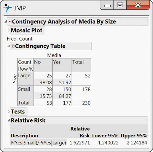
In Example 8.12, the confidence interval is clearly not symmetric about the estimate; that is, 1.62 is much closer to 1.24 than it is to 2.12. This is true, in general, for confidence intervals for relative risk.

Relative risk, comparing proportions by a ratio rather than by a difference, is particularly useful when the proportions are small. This way of describing results is often used for epidemiology and medical studies.