The theory of competition is an extension of logistic growth models

You may recall from Chapter 12 that population growth and regulation can be modeled using the logistic growth equation. Extensions of this equation can help us understand the population dynamics of two species that are competing with each other. In this section, we will begin by examining Lotka-Volterra competition models when there is a single limiting resource. We will then expand our perspective and consider models that include multiple limiting resources. Although these models represent conditions that are simplified from nature, they provide a useful foundation for exploring competitive interactions and the conditions under which species can coexist.

Competition For a Single Resource

To understand how the populations of two species compete for a single resource, let’s begin with the logistic growth equation introduced in Chapter 12:

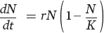
As you may recall, the part of the equation in parentheses represents intraspecific competition for resources. As the size of the population, N, approaches the carrying capacity of the environment, K, the term in parentheses approaches zero. At this point, the population’s growth rate is zero, which means that the population has achieved a stable equilibrium.

If we wish to use this equation to model competition between two species that compete for a single resource, we need to consider the carrying capacity of the environment relative to the number of individuals from both species that are being supported. For example, imagine an environment that has a carrying capacity of 100 rabbits. Let’s also assume that the food needed to support 100 rabbits could instead support 200 squirrels. The environment could also support many different combinations of rabbits and squirrels, such as 90 rabbits and 20 squirrels or 80 rabbits and 40 squirrels.

To include a second species in our equation, we need to add two pieces of information: the number of individuals of the second species and how much each individual of the second species affects the carrying capacity of the first species. For example, if we wanted to know the growth rate of a rabbit population, we would need to know the number of rabbits and squirrels in the area, and—in terms of resource consumption—how many squirrels equal one rabbit. Given that we want to model the changes in population for two species, we will use one equation for each. In these equations, we denote species 1 and 2 using the subscripts 1 and 2, respectively.

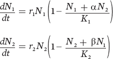
The first equation tells us that the rate of change in the population of species 1 depends on its intrinsic rate of growth (r), the number of individuals of species 1 that are present (N₁), and—in parentheses—the combined effects of species 1 and species 2 in consuming the resource relative to the carrying capacity. The second equation tells us the same thing for species 2.

In these equations, we use two variables, the terms α and β, which are called competition coefficients. Competition coefficients are variables that convert between the number of individuals of one species and the number of individuals of the other species. In the preceding equations, α converts individuals of species 2 into the equivalent number of individuals of species 1. Similarly, β converts individuals of species 1 into the equivalent number of individuals of species 2. In our example of rabbits and squirrels competing for a common food resource, we can define rabbits as species 1 and squirrels as species 2. In that case, the value of α would be 0.5 because one squirrel is equivalent to 0.5 rabbits. Similarly, the value of β would be 2.0 because one rabbit is equivalent to two squirrels.

Graphing the Populations of Each Species at Equilibrium

Using these two equations, we can create graphs that help us understand when each of the populations will reach the point at which it no longer increases or decreases. This point is the population’s equilibrium point. We can start by determining the conditions under which species 1 will have a population at equilibrium. This will happen whenever the change in population size per unit time is zero:

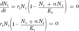
There are two conditions that can make this equation be at equilibrium. One condition occurs when N₁ = 0. Not surprisingly, if we have no individuals of species 1, there will be no growth of species 1. When N₁ is not zero, we can find equilibrium by rearranging the equation:

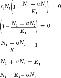
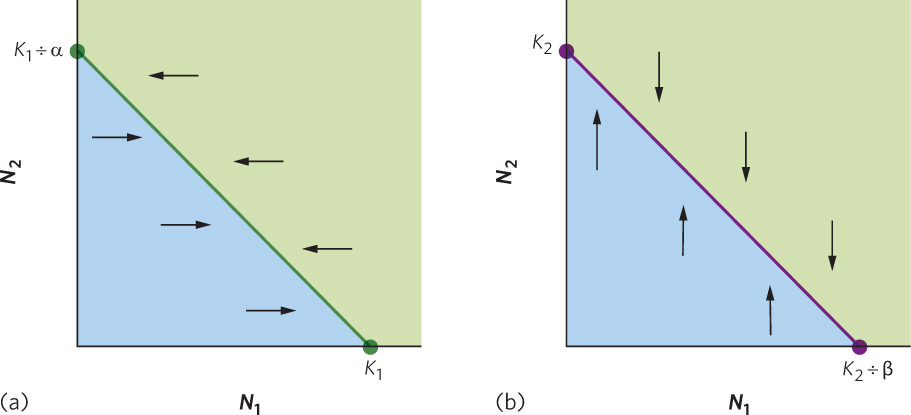
In words, this equation tells us that the number of N₁ individuals depends on the total carrying capacity for species 1 minus the amount of resources consumed by some number of N₂ individuals. Based on this equation, we can draw a line that represents all combinations of N₁ and N₂ that would exist when the N₁ population is at equilibrium. We can plot this line on a graph that has N₁ on the x axis and N₂ on the y axis, as shown in Figure 16.7a. To draw this line, we need to identify the x and y intercepts on the graph.

Figure 16.7 Equilibrium population sizes of two species. (a) The equilibrium isocline for species 1, shown as a green line, represents all combinations of species 1’s population sizes (N₁) and species 2’s population sizes (N₂) that cause species 1 to experience zero growth. When species 2 has an abundance of zero, species 1 will have an abundance of K₁, which is the carrying capacity of species 1. (b) The equilibrium isocline for species 2, shown as a purple line, represents all combinations of species 1’s population sizes (N₁) and species 2’s population sizes (N₂) that cause species 2 to experience zero growth. When species 1 has an abundance of zero, species 2 will have an abundance of K₂, which is the carrying capacity of species 2. The arrows indicate how each population either increases or decreases as it moves away from the equilibrium line.

The x intercept can be found by setting N₂ equal to zero. If we do this, the equation simplifies to

As you can see from this equation, when there are no N₂ individuals, the N₁ population achieves equilibrium when it reaches its carrying capacity, K₁.

The y intercept can be found by setting N₁ equal to zero. If we do this, the equation simplifies to

As you can see from this equation, when there are no N₁ individuals, equilibrium occurs when the N₂ population reaches K₁ ÷ α individuals.

Now that we have identified the x and y intercepts, we can construct the line on the graph that represents all combinations of N₁ and N₂ that cause the population of N₁ to be at equilibrium, as illustrated by the green line in Figure 16.7a. As you can see in this figure, as we increase N₂, the equilibrium population size of N₁ becomes smaller because species 2 is now consuming some of the resource that species 1 needs. Because this equation of a straight line represents population sizes which a population experiences zero growth, it is called a zero population growth isocline.

The zero population growth isocline for species 1 represents the values of N₁ that are in equilibrium across a range of N₂ values. As a result, when the N₁ population is to the left of the isocline, as indicated by the blue-shaded region, it will experience population growth, and move to the right until it reaches the isocline. In contrast, when the N₁ population is to the right of the isocline, as indicated by the green-shaded region, it will experience a population decline, thereby moving to the left until it reaches the isocline.

Now that we have graphically represented the zero population growth isocline for species 1, we need to do the same for species 2. To do this, we set the second equation equal to zero and then rearrange the equation:

You might notice that this equation looks very similar to the equation we derived for N₁. To determine the x and y intercepts for the equilibrium line of species 2, we can go through the same mathematical steps that we used for species 1. For example, when we set N₁ = 0, equilibrium will occur for species 2 when it reaches its carrying capacity:

If we then set N₂ = 0, equilibrium will occur when

Using these two intercepts, we can plot a zero population growth isocline for species 2, as illustrated by the purple line in Figure 16.7b. As you can see in this figure, as N₁ increases, the equilibrium population size of N₂ decreases because species 1 is consuming the resource that species 2 needs. Because this is a zero population growth isocline for species 2, when the N₂ population is above the isocline, as indicated by the green-shaded region, it will experience a population decline until it reaches the isocline. In contrast, when the population is below the isocline, as indicated by the blue-shaded region, it will experience population growth until it hits the isocline.

In drawing both of these population isoclines, you might notice that the growth rates of the two populations (r₁ and r₂) have no effect on the position of the isocline. While the growth rates determine how quickly a population can reach an equilibrium, they do not affect the location of the equilibrium.

Predicting the Outcome of Competition

Now that we know the conditions under which each of two species reaches an equilibrium population size, we can determine if one of the two species will win the competitive interaction or if the two species will coexist. We do this by overlapping the two zero population growth isoclines for species 1 and species 2. As illustrated in Figure 16.8, overlaying the two lines can produce four possible outcomes. In all four cases, when both species start with small population sizes, as indicated by the yellow-shaded region, both species will experience population growth. In contrast, when both species start with large population sizes, as indicated by the green-shaded region, both species will experience a population decline. However, it is the region that lies between these two extremes where we can determine the outcome of competition.

Figure 16.8 Predicting the outcome of competition for a single resource. Based on the Lotka-Volterra competition equations, there are four possible outcomes of competition. (a) If the zero population growth isocline for species 1 is farther out than species 2, species 1 will increase to its carrying capacity and species 2 will go extinct. (b) If the isocline for species 2 is farther out than species 1, species 2 will increase to its carrying capacity and species 1 will go extinct. (c) If the isoclines cross and the two carrying capacities are the outermost points on the two axes, the winner depends on the initial number of each species. (d) If the isoclines cross and the two carrying capacities are the innermost points on the two axes, then the two species will coexist. As in Figure 16.7, the green line represents the population isocline for species 1 and the purple line represents the population isocline for species 2. The thin black arrows represent increases and decreases in population sizes for each species whereas the thick black arrows represent the net effects of population changes in both species.

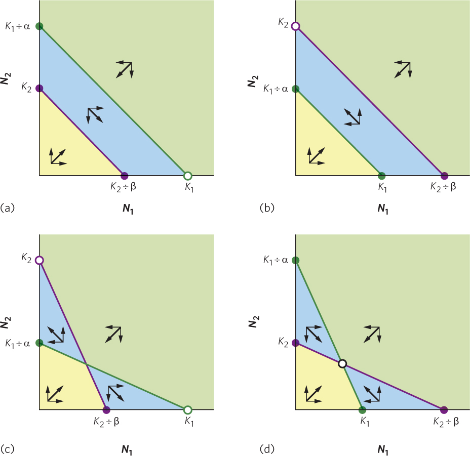
In Figure 16.8a, the isocline for species 1 lies farther out than the isocline for species 2. As a result, any combination of the two species numbers that falls within the blue-shaded region means that species 1 is below its isocline and its population will grow whereas species 2 is above its isocline and its population will decline. The net effect of species 1 moving to the right and species 2 moving down—both indicated by thin arrows—is that the combination of the two species moves down and to the right, as indicated by the thick arrow. This combination will continue to move until eventually it reaches an equilibrium. At this point, N₁ reaches its carrying capacity and N₂ goes extinct.

In Figure 16.8b, we see the opposite situation; the isocline for species 2 lies farther out than the isocline for species 1. In this case, any combination of the two species that falls within the blue-shaded region means that species 1 is above its isocline and its population will decline whereas species 2 is below its isocline and its population will grow. With species 1 moving to the left and species 2 moving up, the net effect is that the combination of the two species moves up and to the left. As this process continues, the combination will reach an equilibrium; N₂ reaches its carrying capacity and N₁ goes extinct.

In Figure 16.8c, the two isoclines cross, with K₁ and K₂ as the two most extreme points on the axes. In this scenario, there are two possible equilibria and the outcome depends on the initial number of each species. If the combination of the two species falls within the blue-shaded region, the outcome of competition depends on the combination of N₁ and N₂ that are present. If the combination of N₁ and N₂ fall within the upper left blue region, the net movement is toward K₂ and species 2 wins the competitive interaction. If the combination of N₁ and N₂ fall within the lower right blue region, the net movement is toward K₁ and species 1 wins.

In Figure 16.8d, the two isoclines also cross, but this time with K₁ and K₂ as the two innermost points on the axes. In this scenario, the movement of each population relative to its respective isocline causes a net movement toward a single equilibrium point where the two lines cross. This means that the two competing species will coexist; one species will not outcompete the other.

In general, these equations tell us that coexistence of two competing species is most likely when interspecific competition is weaker than intraspecific competition—that is, when the competition coefficients α and β are less than 1. In other words, coexistence of two competing species occurs when individuals of each species compete more strongly with themselves (conspecifics) than with individuals of other species (heterospecifics).

Competition for Multiple Resources

Although it is simpler to think about two species competing for one resource, in reality species in nature compete for multiple resources. For example, grassland plants might simultaneously compete for water, nitrogen, and sunlight. We can predict the outcome of this more complex competition by thinking about a case in which two species compete for two different resources. If species 1 is better able to sustain itself at low levels of both resources than species 2, then species 1 will win the competitive interaction. However, the outcome changes when species 1 is better at persisting at a low level of one resource but species 2 is better at persisting at a low level of another resource. In this case, because neither species can drive the other to extinction, the two species should coexist.

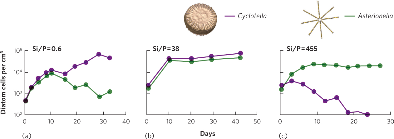
This principle was first demonstrated by David Tilman in a series of experiments conducted with two species of diatoms: Asterionella formosa and Cyclotella meneghiniana. We encountered these species when we discussed Liebig’s law of the minimum. Both species require silica (Si) to produce their glassy outer shells and both species require phosphorus (P) for their metabolic activities. However, each species differs in how much of each resource it needs. Cyclotella uses silicon more efficiently, so its population can persist when there is a low abundance of silicon. In contrast, Asterionella utilizes phosphorus more efficiently, so its population can persist when there is a low abundance of phosphorus. Based on these differences, Tilman predicted that if the diatoms were raised under a low ratio of Si/P, Cyclotella would dominate the competitive interaction because silicon would be low in abundance. If they were raised under a high ratio of Si/P, Asterionella would dominate the competitive interaction because phosphorus would be low in abundance. He also predicted that at intermediate ratios of Si/P, the two species would coexist because each is limited by a different resource.

To test this hypothesis, Tilman raised the two species separately and together under a range of different Si/P ratios in laboratory containers, as shown in Figure 16.9. When raised separately, both species were able to survive under all of the Si/P ratios. However, Cyclotella dominated the containers when they were raised together at a low Si/P ratio of 0.6, while Asterionella dominated the containers when they were raised at a high Si/P ratio of 455. In contrast, when they were raised at an intermediate Si/P ratio of 38, the two species coexisted and neither became dominant. These were the first results to demonstrate that competing species can coexist when there are multiple resources and each species is limited by a different resource.

Figure 16.9 Species competing for multiple resources. In the experiment, two species of diatoms compete for silicon and phosphorus. Cyclotella is more limited by a low abundance of phosphorus whereas Asterionella is more limited by a low abundance of silicon. (a) When raised under a low ratio of Si/P, Cyclotella dominates the competitive interaction. (b) When raised under an intermediate ratio of Si/P, neither species dominates. Instead, the two species coexist. (c) When raised under a high ratio of Si/P, Asterionella dominates the competitive interaction.

Data from D. Tilman, Resource competition between planktonic algae: An experimental and theoretical approach, Ecology 58 (1977): 338–348.