How Do We Study Earthquakes?

As in any experimental science, instruments and field observations provide the basic data used to study earthquakes. These data enable investigators to locate earthquakes, determine their sizes and numbers, and understand their relationships to faults.

Seismographs

The seismograph, an instrument that records the seismic waves, is to the Earth scientist what the telescope is to the astronomer: a tool for peering into inaccessible regions (Figure 13.8). The ideal seismograph would be a device affixed to a stationary frame that is not attached to Earth. When the ground shook, the seismograph would measure the changing distance between the frame, which did not move, and the vibrating ground, which did. As yet, we have no way to position a seismograph that is not attached to Earth—although Global Positioning System (GPS) technology is beginning to remove this limitation. So we compromise. We attach a dense mass, such as a piece of steel, to Earth so loosely that the ground can vibrate up and down or side to side without causing much movement of the mass.

Figure 13.8: A seismograph consists of a dense mass (such as a steel ball) attached to a recording device. Because of its inertia and its loose coupling to Earth through (a) a spring or (b) a hinge, the mass does not keep up with the motion of the ground.

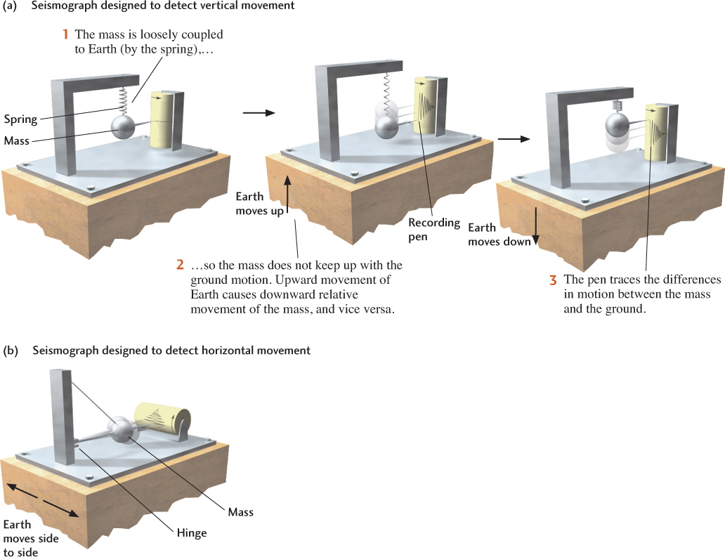
This loose attachment can be achieved by suspending the mass from a spring (Figure 13.8a). When seismic waves move the ground up and down, the mass tends to remain stationary because of its inertia (an object at rest tends to stay at rest), but the mass and the ground move relative to each other because the spring can compress or stretch. In this way, the vertical displacement of the ground caused by seismic waves can be recorded by a pen on chart paper or, almost always these days, digitally on a computer. Such a record is called a seismogram.

Loose attachment of the mass can also be achieved with a hinge. A seismograph that has its mass suspended on hinges, like a swinging gate (Figure 13.8b), can record the horizontal displacement of the ground.

A typical seismographic station has seismographs set up to measure three components of ground movement: vertical, horizontal east-west, and horizontal north-south. Modern seismographs can detect ground oscillations of less than a billionth of a meter—an astounding feat, considering that such small displacements are of atomic size!

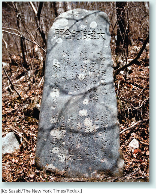
Earth Issues: 13.1 The Tsunami Stone of Aneyosh

On a hill along the Tohoku coastline of northeastern Honshu, in the fishing hamlet of Aneyoshi, sits a stone monument of uncertain age, inscribed with Japanese characters that read, “High dwellings are the peace and harmony of our descendants. Remember the calamity of the great tsunamis. Do not build any homes below this point.” Aneyoshi, now part of the city of Miyako, was once more conveniently located down by the sea where the fishermen tied their boats, but only four of its residents survived the tsunami of 1896 and only two survived the tsunami of 1933. The stone reminds people why they now live on higher ground.

History became prophecy at 2:46 p.m. on March 11, 2011, when the offshore thrust fault that separates Japan from the Pacific plate began to slip. The rupture started on a small patch of the fault surface 30 kilometers beneath the ocean, about 100 km southeast of Aneyoshi, and accelerated outward like a crack through glass, reaching speeds of nearly 3 km/s (more than 6000 miles/hour). By the time it stopped several minutes later, the Pacific Plate had moved under Japan by as much as 40 m along a fault surface the size of South Carolina. Seismic waves from this Tohoku megaquake, which measured magnitude 9, propagated over Earth’s surface and through its deep interior, causing the planet to ring like a bell for many days.

The thrusting of Honshu eastward and upward over the Pacific plate raised the seafloor as much as 10 m almost instantly, displacing several hundred billion tons of water, which flowed away from the fault in a huge tsunami. In less than an hour, the water waves, slower than the seismic waves but much more deadly, passed into the bays and inlets of the Japanese coastline like an undulating monster, gaining height as they approached the shore. Funneled into harbors, the waves created immense walls of water—tsunami is Japanese for “harbor wave”—which inundated the near-shore communities, sweeping up boats, cars, and buildings, in some places travelling several kilometers inland.

The fast-moving swath of devastation was captured on horrific videos from helicopters overhead and by survivors who made it to high ground and the tops of buildings. The tsunami overran the seawalls designed to protect the city center of Miyako, destroying all but 30 of the 1,000 boats in its famous fishing fleet and killing many hundreds who could not, or did not, escape in time. Though the exact number remains uncertain, the death toll along the Tohoku coastline was almost 20,000. One of the highest levels reached by the enormous wave—the greatest in recent Japanese history—was 39 m (128 ft) above the shoreline, just below the Aneyoshi tsunami stone. The residents in their houses above the stone were safe.

The tsunami stone at Aneyoshi.

Seismic Waves

Install a seismograph almost anywhere, and within a few hours it will record the passage of seismic waves generated by an earthquake somewhere on Earth. The waves travel from the earthquake focus through Earth and arrive at the seismograph in three distinct groups (Figure 13.9a). The first waves to arrive are called primary waves, or P waves. The secondary waves, or S waves, follow. Both P waves and S waves travel through Earth’s interior. Afterwards come the slower surface waves, which travel around Earth’s surface.

Figure 13.9: (a) The three types of waves travel by different routes and at different speeds to a seismograph that records them. (b) The three types of seismic waves are characterized by distinct types of ground deformation. The red squares show the distortion of a section of rock as a wave passes through it.

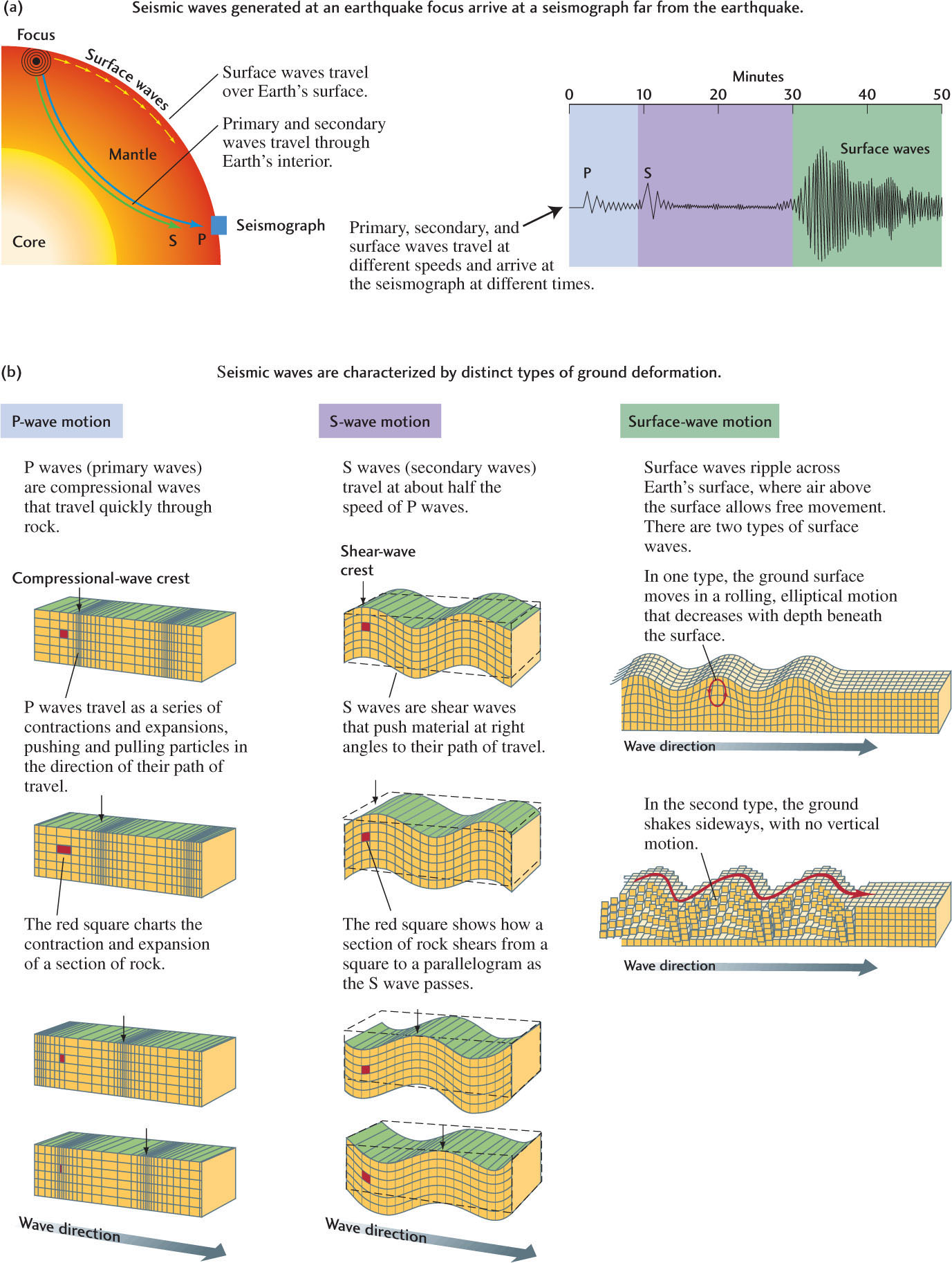
P waves in rock are similar to sound waves in air, except that P waves travel through the solid rock of Earth’s crust at about 6 km/s, which is about 20 times faster than sound waves travel through air. Like sound waves, P waves are compressional waves, so called because they travel through solid, liquid, or gaseous materials as a succession of compressions and expansions (Figure 13.9b). P waves can be thought of as push-pull waves: they push or pull particles of matter in the direction of their path of travel.

S waves travel through solid rock at a little more than half the velocity of P waves. They are shear waves that displace material at right angles to their path of travel (see Figure 13.9b). Shear waves cannot travel through liquids or gases.

The velocities at which P and S waves travel are higher when the resistance to their movement is greater. It takes more force to compress solids than to shear them, so P waves always travel faster than S waves through a solid, which is why the P waves from an earthquake arrive at a seismograph before the S waves. This physical principle also explains why S waves cannot travel through air, water, or Earth’s liquid outer core: gases and liquids put up no resistance to shear.

Surface waves are confined to Earth’s surface and outer layers, like waves on the ocean. Their velocity is slightly less than that of S waves. One type of surface wave sets up a rolling motion in the ground; another type shakes the ground sideways (see Figure 13. 9b). Surface waves are usually the most destructive waves in a large, shallow-focus earthquake, especially in sedimentary basins, where reverberations in the soft near-surface sediments can increase their amplitudes, causing much stronger shaking than in the basement rocks.

People have felt seismic waves and witnessed their destructiveness throughout history, but not until the close of the nineteenth century were scientists able to devise seismographs to record them accurately. Seismic waves enable us to study earthquakes but also provide our most important means of probing Earth’s deep interior, as we will see in Chapter 14.

Locating the Focus

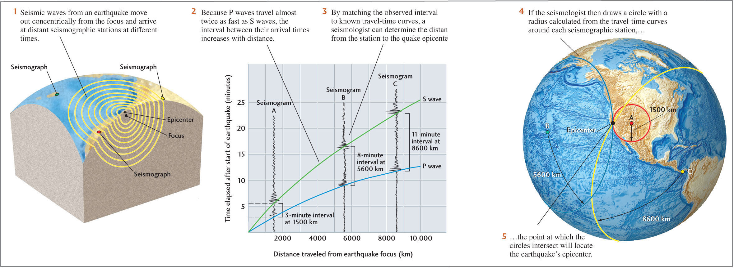
Locating an earthquake’s focus is like deducing the distance of a lightning strike from the time interval between the flash of light and the sound of thunder: the greater the distance to the lightning bolt, the longer the time interval. Light travels faster than sound, so the lightning flash may be likened to the P waves of an earthquake and the thunder to the slower S waves.

The time interval between the arrival of P waves and S waves depends on the distance the waves have traveled from the focus: the longer the interval, the longer the distance the waves have traveled. Seismologists have used networks of sensitive seismographs around the world and highly accurate clocks to time the arrival of seismic waves from earthquakes as well as from underground nuclear test sites at known locations. From the results, they have constructed travel-time curves, which show how long it takes seismic waves of each type to travel a certain distance.

To estimate the distance to a new quake’s focus, seismologists read from a seismogram the amount of time between the arrival of the first P waves and the arrival of the first S waves. Then they use travel-time curves, like the ones shown in Figure 13.10, to determine the distance from the seismograph to the focus. If they can determine the distances from three or more seismographic stations, they can locate the focus (see Figure 13.10). They can also deduce the time of the quake at the focus—the earthquake’s origin time—-because the arrival time of the first P waves at each station is known, and it is possible to determine from the travel-time curves how long those waves took to reach the station. Today, this entire process is done automatically by computers, which use data from a large network of seismographs to determine each earthquake’s epicenter, depth of focus, and origin time.

Figure 13.10: Readings from three or more seismographic stations can be used to determine the location of an earthquake’s focus.

Measuring the Size of an Earthquake

Locating earthquakes is only one step on the way to understanding them. We must also determine their sizes, or magnitudes. Other things being equal (such as distance from the focus and regional geology), an earthquake’s magnitude is the main factor that determines the intensity of the seismic waves it produces, and thus the earthquake’s potential destructiveness.

Richter Magnitude

In 1935, Charles Richter, a California seismologist, devised a simple procedure that assigned a numerical size to each earthquake, now called the Richter magnitude (Figure 13.11). Richter studied astronomy as a young man and learned how astronomers use a logarithmic scale to measure the brightnesses of stars, which vary over a huge range of values. Adapting this idea to earthquakes, Richter took as his measure of earthquake size the logarithm of the largest ground movement registered by a standard type of seismograph at a standard distance, thus defining a magnitude scale.

Figure 13.11: The maximum amplitude of ground movement, corrected by the P-S wave interval, is used to assign a Richter magnitude to an earthquake.

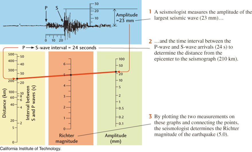
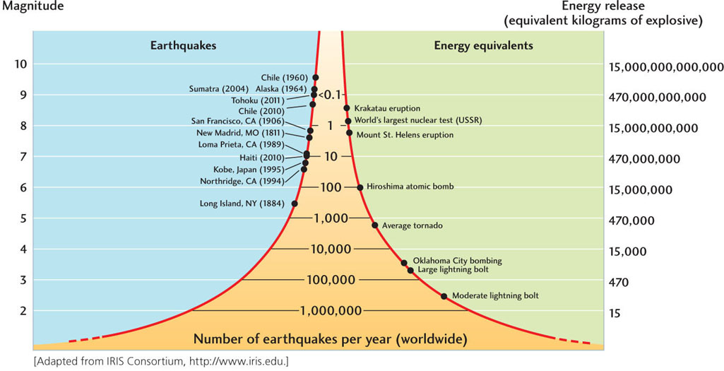
On Richter’s magnitude scale, two earthquakes at the same distance from a seismograph differ by one magnitude unit if the peak amplitude of the ground movement they produce differs by a factor of 10. The ground movement of an earthquake of magnitude 3, therefore, is 10 times that of an earthquake of magnitude 2. Similarly, a magnitude 6 earthquake produces ground movements that are 100 times greater than those of a magnitude 4 earthquake. The energy released as seismic waves increases even more with earthquake magnitude, by a factor of about 32 for each magnitude unit. A magnitude 7 earthquake releases 32 ✕ 32, or about 1000, times the energy of a magnitude 5 earthquake. According to this energy scale, the Tohoku megaquake was a million times more powerful than a magnitude 5 event!

Seismic waves gradually weaken as they move away from the focus, so to make his procedure work for any seismograph, Richter had to find a way to correct the measurement of ground movement for the distance between the seismograph and the focus. He devised a simple graph that allowed seismologists at different locations to quickly come up with nearly the same value for the magnitude of an earthquake no matter how far their instruments were from the focus (see Figure 13.11). His procedure came to be used throughout the world.

Moment Magnitude

Although “Richter scale” has become a household term, seismologists prefer a measure of earthquake size more directly related to the physical properties of the faulting that causes an earthquake. The seismic moment of an earthquake is defined as a number proportional to the product of the area of faulting and the average fault slip. The corresponding moment magnitude increases by about one unit for every tenfold increase in the area of faulting (see the Practicing Geology exercise at the end of the chapter).

Although Richter’s method and the moment method produce roughly the same numerical values, the moment magnitude can be measured more accurately from seismographs, and it can sometimes be determined directly from field measurements of the fault.

Magnitude and Frequency

Large earthquakes occur much less often than small ones. This observation can be expressed by a simple relationship between earthquake frequency and magnitude (Figure 13.12). Worldwide, approximately 1,000,000 earthquakes with magnitudes greater than 2 take place each year. This number decreases by a factor of 10 for each magnitude unit. Hence, there are about 100,000 earthquakes with magnitudes greater than 3, about 1000 with magnitudes greater than 5, and about 10 with magnitudes greater than 7 each year.

Figure 13.12: Relationship between moment magnitude, seismic energy release, and number of earthquakes per year worldwide. Examples of earthquakes of various magnitudes and of other large sources of sudden energy release are included for comparison.

According to these statistics, there should be, on average, about 1 earthquake with a magnitude greater than 8 per year and 1 earthquake with a magnitude greater than 9 every 10 years. In fact, the very largest earthquakes, such as the ones that occurred on thrust faults in the subduction zones off Japan in 2011 (moment magnitude 9.0), Sumatra in 2004 (moment magnitude 9.2), Alaska in 1964 (moment magnitude 9.1), and Chile in 1960 (moment magnitude 9.5) and 2010 (moment magnitude 8.8) are almost this common when averaged over many decades. However, even the largest subduction zone megathrusts are too small to create magnitude 10 earthquakes, so seismologists believe that events of such extreme size do not follow this rule; that is, they are less frequent than once per century.

Shaking Intensity

Earthquake magnitude by itself does not describe seismic hazard because the shaking that causes destruction generally weakens with distance from the fault rupture. A magnitude 8 earthquake in a remote area far from the nearest city might cause no human or economic losses, whereas a magnitude 6 quake immediately beneath a city would likely cause serious damage. The destruction in Christchurch by the earthquakes of February 22 and June 13, 2011, illustrates this important point (see Figure 13.7).

In the late nineteenth century, before Richter invented his magnitude scale, seismologists and earthquake engineers developed intensity scales for estimating the intensity of shaking directly from an earthquake’s destructive effects. Table 13.1 shows one intensity scale that remains in common use today, called the modified Mercalli intensity scale after Giuseppe Mercalli, the Italian scientist who proposed it in 1902. This scale assigns a value, given as a Roman numeral from I to XII, to the intensity of the shaking at a particular location. For example, a location where an earthquake is barely felt by a few people is assigned an intensity of II, whereas one where it was felt by nearly everyone is assigned an intensity of V. Numbers at the upper end of the scale indicate increasing amounts of damage. The narrative attached to the highest value, XII, is tersely apocalyptic: “Damage total. Lines of sight and level are distorted. Objects thrown into the air.”

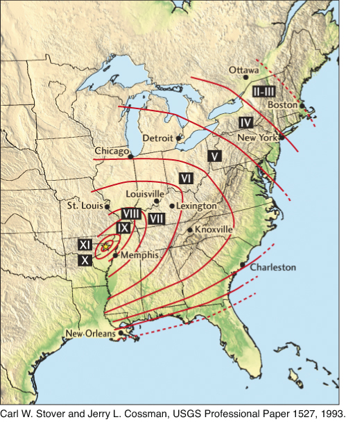
By making observations at many sites and interviewing many people who experienced an earthquake, or even by examining historical records, seismologists can make maps showing contours of equal shaking intensity. Figure 13.13 shows an intensity map for the New Madrid earthquake of December 16, 1811, a magnitude 7.7 event near the southern tip of Missouri, which was felt as far away as Boston. Although earthquake intensities are generally highest near the fault rupture, they also depend on the local geology. For example, when sites at equal distances from the rupture are compared, the shaking tends to be more intense on soft sediments (especially water-saturated sediments near shorelines) than on hard basement rock. Intensity maps thus provide engineers with crucial data for designing structures to withstand seismic shaking.

Figure 13.13: Measurements of modified Mercalli intensities for the New Madrid earthquake of December 16, 1811, a magnitude 7.7 event near the juncture of Missouri, Arkansas, and Tennessee. Regions near the epicenter experienced intensities greater than IX, and intensities as high as VI were observed 200 km from the epicenter (see Table 13.1).

Determining Fault Mechanisms

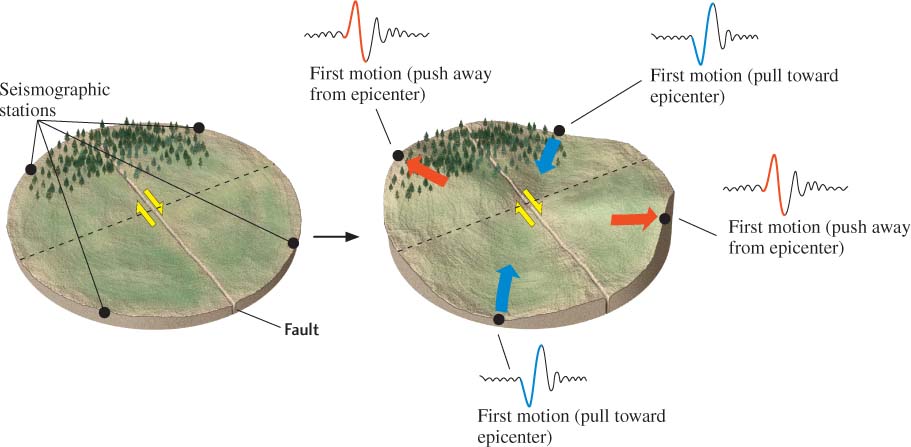
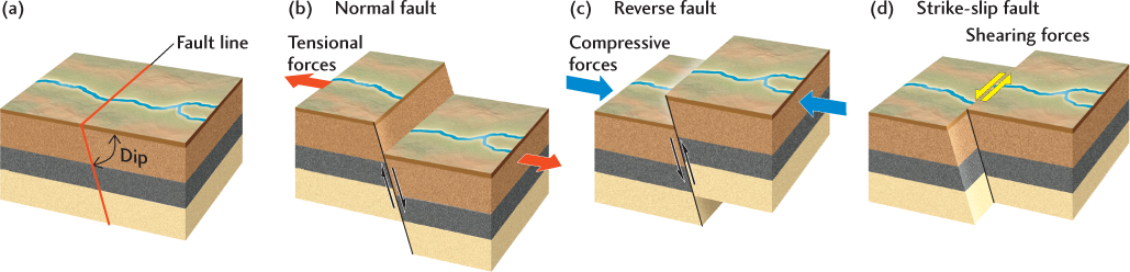
The pattern of ground shaking also depends on the orientation of the fault rupture and the direction of slipping, which together specify the fault mechanism of an earthquake. The fault mechanism tells us whether the rupture was on a normal, reverse, or strike-slip fault. If the rupture was on a strike-slip fault, the fault mechanism also tells us whether the movement was right-lateral or left-lateral (see Figure 7.8 for the definitions of these terms). We can then use this information to infer the regional pattern of tectonic forces (Figure 13.14).

Figure 13.14: The three main types of fault mechanisms that initiate earthquakes and the stresses that cause them. (a) A fault before movement takes place. (b) Normal faulting due to tensional stress. (c) Reverse faulting due to compressive stress. (d) Strike-slip faulting due to shearing stress (in this case, left-lateral).

For shallow ruptures that break the surface, we can sometimes determine the fault mechanism from field observations of the fault scarp. As we have seen, however, most ruptures are too deep to break the surface, so we must deduce the fault mechanism from seismograms.

For large earthquakes at any depth, this task turns out to be easy, because there are enough seismographic stations around the world to surround any earthquake’s focus. In some directions from the focus, the very first movement of the ground recorded by a seismograph—a P wave—is a push away from the focus, causing upward movement on a vertical seismograph. In other directions, the initial ground movement is a pull toward the focus, causing downward movement on a vertical seismograph. For strike-slip ruptures, the directions of the largest pushes lie on an axis rotated 45º from the fault plane and are perpendicular to the directions of the largest pulls (Figure 13.15). The locations of pushes and pulls can therefore be plotted and divided into four sections based on the positions of the seismographic stations. One of the two boundaries between those sections will be the fault orientation; the other will be a plane perpendicular to the fault. The slip direction on the fault plane can also be determined from the arrangement of pushes and pulls. In this manner, without surface evidence, seismologists can deduce whether the horizontal crustal forces that triggered an earthquake were tensional, compressive, or shearing forces.

Figure 13.15: The movement marking the first P wave arriving from a fault rupture at each of several seismographic stations is used to determine the orientation of the fault and the direction of fault slipping. The case shown here is the rupture of a right-lateral strike-slip fault. Note that the alternating pattern of pushes and pulls would remain the same if a plane perpendicular to the fault ruptured with left-lateral displacement. Seismologists can usually choose between the two possibilities using additional information, such as field mapping of the fault scarp or the alignment of aftershocks along the fault.