16.1 The Economics of Pollution
Pollution is a bad thing. Yet most pollution is a side effect of activities that provide us with good things: our air is polluted by power plants generating the electricity that lights our cities, and our rivers are damaged by fertilizer runoff from farms that grow our food. Why shouldn’t we accept a certain amount of pollution as the cost of a good life?
The marginal social cost (MSC) of pollution is the additional cost imposed on society as a whole by an additional unit of pollution.
Actually, we do. Even highly committed environmentalists don’t think that we can or should completely eliminate pollution—
The marginal social benefit (MSB) of pollution is the additional gain to society as a whole from an additional unit of pollution.
The marginal private cost (MPC) of pollution is the additional cost imposed on the polluter if the polluter creates another unit of pollution.
The marginal external cost (MEC) of pollution is the additional cost imposed on others if the polluter creates another unit of pollution.
To see why, we need a framework that lets us think about how much pollution a society should have. We’ll then be able to see why a market economy, left to itself, will produce more pollution than it should. We’ll start by adopting the simplest framework to study the problem—
Costs and Benefits of Pollution
How much pollution should society allow? We learned in Chapter 9 that “how much” decisions always involve comparing the marginal benefit from an additional unit of something with the marginal cost of that additional unit. The same is true of pollution.
The marginal social cost (MSC) of pollution is the additional cost imposed on society as a whole by an additional unit of pollution. For example, acid rain damages fisheries, crops, and forests, and each additional tonne of sulphur dioxide released into the atmosphere increases the damage.
The marginal social benefit (MSB) of pollution—the additional benefit to society from an additional unit of pollution—
SO HOW DO YOU MEASURE THE MARGINAL SOCIAL COST OF POLLUTION?
It might be confusing to think of marginal social cost—
But calculating the true cost to society of pollution—
The marginal social cost of pollution can be expressed as the sum of two terms (MSC = MPC + MEC): marginal private cost (MPC) of pollution—the additional cost imposed on the polluter if the polluter creates another unit of pollution—
Similarly, the marginal social benefit is the sum of two terms (MSB = MPB + MEB): marginal private benefit (MPB) of pollution—the additional benefit the polluter receives if the polluter creates another unit of pollution—
The marginal private benefit (MPB) of pollution is the additional benefit the polluter receives if the polluter creates another unit of pollution.
Using hypothetical numbers, Figure 16-1 shows how we can determine the socially optimal quantity of pollution—the quantity of pollution society would choose if all its costs and benefits were fully accounted for. The upward-
The marginal external benefit (MEB) of pollution is the additional benefit others receive if the polluter creates another unit of pollution.
The socially optimal quantity of pollution is the quantity of pollution that society would choose if all the costs and benefits of pollution were fully accounted for.
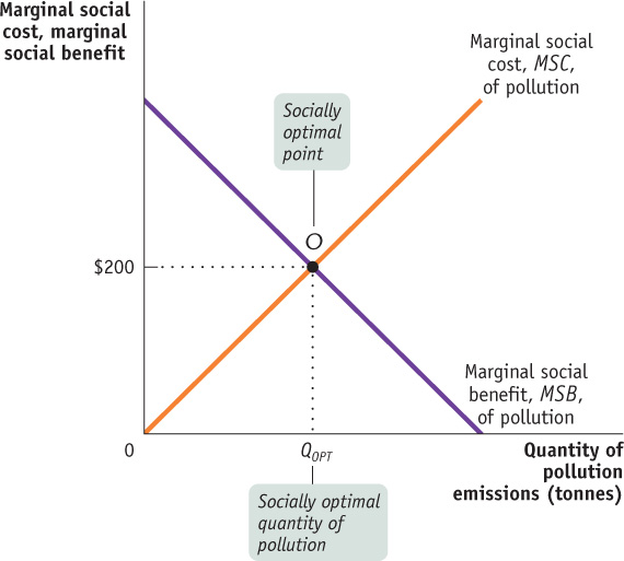
The socially optimal quantity of pollution in this example isn’t zero. It’s QOPT, the quantity corresponding to point O, where MSB crosses MSC. At QOPT, the marginal social benefit from an additional tonne of emissions and its marginal social cost are equalized at $200.
But will a market economy, left to itself, arrive at the socially optimal quantity of pollution? No, it won’t.
SO HOW DO YOU MEASURE THE MARGINAL SOCIAL BENEFIT OF POLLUTION?
Similar to the problem of measuring the marginal social cost of pollution, the concept of willingness to pay helps us understand the marginal social benefit of pollution in contrast to the marginal benefit to an individual or firm. The marginal social benefit of a unit of pollution is simply equal to the highest willingness to pay for the right to emit that unit measured across all polluters. But unlike the marginal social cost of pollution, the value of the marginal social benefit of pollution is a number likely to be known—
Pollution: An External Cost
Pollution yields both benefits and costs to society. But in a market economy without government intervention, those who benefit from pollution—
To see why, remember the nature of the benefits and costs from pollution. For polluters, the benefits take the form of monetary savings: by emitting an extra tonne of sulphur dioxide, any given polluter saves the cost of buying expensive, low-
The costs of pollution, though, fall on people who have no say in the decision about how much pollution takes place: for example, about half of all airborne sulphur dioxide in eastern Canada comes from sources in the United States, especially coal burning power plants in and around the Tennessee Valley. People who fish in Canada do not control the decisions of power plants in Tennessee. (This means MPC = 0, so MSC = MEC > 0. A competitive market equilibrium will be where MPB = MPC = 0, which means too much pollution will be created.)
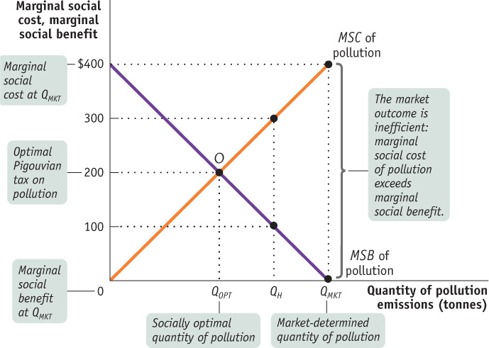
Figure 16-2 shows the result of this asymmetry between who reaps the benefits and who pays the costs. In a market economy without government intervention to protect the environment, only the benefits of pollution are taken into account in choosing the quantity of pollution. So the quantity of emissions won’t be the socially optimal quantity QOPT; it will be QMKT, the quantity at which the marginal social benefit of an additional tonne of pollution is zero, but the marginal social cost of that additional tonne is much larger—
TALKING, TEXTING, AND DRIVING
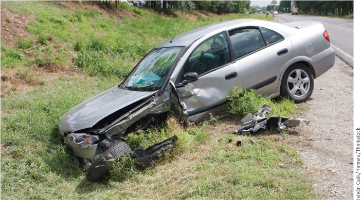
Why is that driver in the car in front of us driving so erratically? Could he or she be drunk? Or falling asleep? No, it turns out the driver is talking on a cellphone or maybe texting.
Traffic safety experts take the risks posed by driving while using a cellphone very seriously: A recent study found a six-
The Canadian Global Road Safety Committee urges people not to use any phones while driving. In response to a growing number of accidents, all Canadian provinces and Yukon have banned the use of all hand-
Why not leave the decision up to the driver? Because the risk posed by driving while using a cellphone isn’t just a risk to the driver; it’s also a safety risk to others—
The reason is that in the absence of government intervention, those who derive the benefits from pollution—
An external cost is an uncompensated cost that an individual or firm imposes on others.
The environmental costs of pollution are the best-
An external benefit is a benefit that an individual or firm confers on others without receiving compensation. External costs and benefits are known as externalities. External costs are negative externalities, and external benefits are positive externalities.
We’ll see later in this chapter that there are also important examples of external benefits, benefits that individuals or firms confer on others without receiving compensation. External costs and benefits are jointly known as externalities with external costs called negative externalities and external benefits called positive externalities.
As we’ve already suggested, externalities can lead to individual decisions that are not optimal for society as a whole. Let’s take a closer look at why.
The Inefficiency of Excess Pollution
We have just shown that in the absence of government action, the quantity of pollution will be inefficient: polluters will pollute up to the point at which the marginal social benefit of pollution is zero, as shown by the pollution quantity, QMKT, in Figure 16-2. Recall that an outcome is efficient if no one could be made better off without making someone else worse off. In Chapter 4 we showed why the market equilibrium quantity in a perfectly competitive market is the efficient quantity of the good, the quantity that maximizes total surplus. Here, we can use a variation of that analysis to show how the presence of a negative externality upsets that result.
Because the marginal social benefit of pollution is zero at QMKT, reducing the quantity of pollution by one tonne would subtract very little from the total social benefit from pollution. In other words, the benefit to polluters from that last unit of pollution is very low—
If the quantity of pollution is reduced further, there will be more gains in total surplus, though they will be smaller. For example, if the quantity of pollution is QH in Figure 16-2, the marginal social benefit of a tonne of pollution is $100, but the marginal social cost is still $300. In other words, reducing the quantity of pollution by one tonne leads to a net gain in total surplus of approximately $300 – $100 = $200. This tells us that QH is still an inefficiently high quantity of pollution. Only if the quantity of pollution is reduced to QOPT, where the marginal social cost and the marginal social benefit of an additional tonne of pollution are both $200, is the outcome efficient.
Externalities and the Competitive Market
Pollution is a by-
Figure 16-3 depicts the market for electricity, which we assume is perfectly competitive. The demand curve represents the marginal social benefit of consuming electricity. Since pollution only imposes additional costs on the rest of society, the industry supply curve is the marginal private cost of producing electricity in perfect competition.
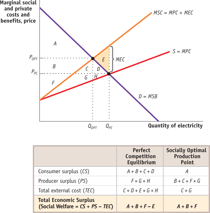
The marginal social cost of electricity production is the sum of the marginal private cost of generating the electricity and the marginal external cost of pollution. That means that the gap between MSC and MPC in the diagram must equal MEC. MSC gets its upward slope partly from the upward-
The perfectly competitive market for electricity is in equilibrium where supply intersects demand at price PPC and quantity QPC. The resulting consumer surplus is the triangle above PPC (below the demand curve). Likewise, the producer surplus is the triangle below PPC (above the supply curve). But unlike the used books we examined in Chapter 4, in this market, the sum of the consumer and producer surplus is not the total benefit to society from the production and consumption of the good—
The socially optimal level of electricity production occurs where MSB intersects MSC. Figure 16-3 reveals that the perfectly competitive equilibrium is inefficient; perfect competition is not socially optimal when there are externalities—
Private Solutions to Externalities
Can the private sector solve the problem of externalities without government intervention? Bear in mind that when an outcome is inefficient, there is potentially a deal that makes people better off. Why don’t individuals find a way to make that deal?
In an influential 1960 article, the economist and Nobel laureate Ronald Coase pointed out that in an ideal world the private sector could indeed deal with all externalities. According to the Coase theorem, even in the presence of externalities an economy can always reach an efficient solution provided that the costs of making a deal are sufficiently low. The costs of making a deal are known as transaction costs.
According to the Coase theorem, even in the presence of externalities an economy can always reach an efficient solution as long as transaction costs—the costs to individuals of making a deal—are sufficiently low.
To get a sense of Coase’s argument, imagine two neighbours, Mick and Christina, who both like to barbecue in their backyards on summer afternoons. Mick likes to play golden oldies on his stereo while barbecuing, but this annoys Christina, who can’t stand that kind of music.
Who prevails? You might think that it depends on the legal rights involved in the case: if the law says that Mick has the right to play whatever music he wants, Christina just has to suffer; if the law says that Mick needs Christina’s consent to play music in his backyard, Mick has to live without his favourite music while barbecuing.
But as Coase pointed out, the outcome need not be determined by legal rights, because Christina and Mick can make a private deal. Even if Mick has the right to play his music, Christina could pay him not to. Even if Mick can’t play the music without an okay from Christina, he can offer to pay her to give that okay. These payments allow them to reach an efficient solution, regardless of who has the legal upper hand. If the benefit of the music to Mick exceeds its cost to Christina, the music will go on; if the benefit to Mick is less than the cost to Christina, there will be silence.
The implication of Coase’s analysis is that externalities need not lead to inefficiency because individuals have an incentive to make mutually beneficial deals—deals that lead them to take externalities into account when making decisions. When individuals do take externalities into account, economists say that they internalize the externality. If externalities are fully internalized, the outcome is efficient even without government intervention.
When individuals take external costs or benefits into account, they internalize the externality.
Why can’t individuals always internalize externalities? Our barbecue example implicitly assumes the transaction costs are low enough for Mick and Christina to be able to make a deal. In many situations involving externalities, however, transaction costs prevent individuals from making efficient deals. Examples of transaction costs include the following:
The costs of communication among the interested parties. Such costs may be very high if many people are involved.
The costs of making legally binding agreements. Such costs may be high if expensive legal services are required.
Costly delays involved in bargaining. Even if there is a potentially beneficial deal, both sides may hold out in an effort to extract more favourable terms, leading to increased effort and forgone benefit.
In some cases, people do find ways to reduce transaction costs, allowing them to internalize externalities. For example, a house with a junk-filled yard and peeling paint imposes a negative externality on the neighbouring houses, diminishing their value in the eyes of potential house buyers. Some people live in private communities that set rules for home maintenance and behaviour, making bargaining between neighbours unnecessary. But in many cases, transaction costs are too high to make it possible to deal with externalities through private action. For example, tens of millions of people are adversely affected by acid rain. It would be prohibitively expensive to try to make a deal among all those people and all those power companies.
When transaction costs prevent the private sector from dealing with externalities, it is time to look for government solutions. We turn to public policy in the next section.

THANK YOU FOR NOT SMOKING
To some they are known as the “shiver-and-puff people”—the smokers who stand outside their workplaces, even in the depths of winter, to take a cigarette break. Over the past couple of decades, rules against smoking in spaces shared by others have become ever stricter. This is partly a matter of personal dislike—non-smokers really don’t like to smell other people’s cigarette smoke—but it also reflects concerns over the health risks of second-hand smoke. As Health Canada’s warning on many packs says, smoking causes lung cancer, heart disease, and strokes, and may complicate pregnancy. And there’s no question that being in the same room as someone who smokes exposes you to at least some health risk.
Second-hand smoke, then, is clearly an example of a negative externality. But how important is it? Putting a dollar-and-cents value on it—that is, measuring the marginal social cost of cigarette smoke—requires not only estimating the health effects but putting a value on these effects. Despite the difficulty, economists have tried. A paper published in 1993 in the Journal of Economic Perspectives surveyed the research on the external costs of both cigarette smoking and alcohol consumption.
According to this paper, valuing the health costs of cigarettes depends on whether you count the costs imposed on members of smokers’ families, including unborn children, in addition to costs borne by smokers. If you don’t, the external costs of second-hand smoke have been estimated at about $0.52 per pack smoked, according to a 2005 study. (This corresponds to the average social cost of smoking per pack at the current level of smoking in society.) If you include effects on smokers’ families, the number rises considerably—family members who live with smokers are exposed to a lot more smoke. (They are also exposed to the risk of fires, which alone is estimated at $0.09 per pack.) If you include the effects of smoking by pregnant women on their unborn children’s future health, the cost is immense—$4.80 per pack, which is more than the pre-tax price charged by cigarette manufacturers.
In 2011, a report issued by Physicians for a Smoke-Free Canada estimated the economic benefit of each smoker who quits: avoiding health care costs of $8553 and $413 000 in benefits from the avoidance of premature deaths—$421 553 in total benefit per smoker who quits. (M. Gross, J. L. Sindelar, J. Mullahy, and R. Anderson, Policy Watch: Alcohol and Cigarette Taxes, Journal of Economic Perspectives, 7, 211-222, 1993.)

Quick Review
The marginal social cost (MSC) of pollution is equal to the sum of the marginal private cost (MPC) of pollution and the marginal external cost (MEC) of pollution: MSC = MPC + MEC
The marginal social benefit (MSB) of pollution is equal to the sum of the marginal private benefit (MPB) of pollution and the marginal external benefit (MEB) of pollution: MSB = MPB + MEB
There are costs as well as benefits to reducing pollution, so the optimal quantity of pollution isn’t zero. Instead, the socially optimal quantity of pollution is the quantity at which MSC = MSB.
Left to itself, a market economy will typically generate an inefficiently high level of pollution because polluters have no incentive to take into account the costs they impose on others.
External costs and benefits are known as externalities. Pollution is an example of an external cost, or negative externality; in contrast, some activities can give rise to external benefits, or positive externalities.
According to the Coase theorem, the private sector can sometimes resolve externalities on its own: if transaction costs aren’t too high, individuals can reach a deal to internalize the externality. When transaction costs are too high, government intervention may be warranted.
Check Your Understanding 16-1
CHECK YOUR UNDERSTANDING 16-1
Question 16.1
Waste water runoff from large poultry farms adversely affects their neighbours. Explain the following:
The nature of the external cost imposed
The outcome in the absence of government intervention or a private deal
The socially optimal outcome
The external cost is the pollution caused by the waste water runoff, an uncompensated cost imposed by the poultry farms on their neighbours.
Since poultry farmers do not take the external cost of their actions into account when making decisions about how much waste water to generate, they will create more runoff than is socially optimal in the absence of government intervention or a private deal. They will produce runoff up to the point at which the marginal social benefit of an additional unit of runoff is zero; however, their neighbours experience a high, positive level of marginal social cost of runoff from this output level. So the quantity of waste water runoff is inefficient: reducing runoff by one unit would reduce total social benefit by less than it would reduce total social cost.
At the socially optimal quantity of waste water runoff, the marginal social benefit is equal to the marginal social cost. This quantity is lower than the quantity of waste water runoff that would be created in the absence of government intervention or a private deal.
Question 16.2
According to Yasmin, any student who borrows a book from the university library and fails to return it on time imposes a negative externality on other students. She claims that rather than charging a modest fine for late returns, the library should charge a huge fine so that borrowers will never return a book late. Is Yasmin’s economic reasoning correct?
Yasmin’s reasoning is not correct: allowing some late returns of books is likely to be socially optimal. Although you impose a marginal social cost on others every day that you are late in returning a book, there is some positive marginal social benefit to you of returning a book late—for example, you get a longer period to use it in working on a term paper.
The socially optimal number of days that a book is returned late is the number at which the marginal social benefit equals the marginal social cost. A fine so stiff that it prevents any late returns is likely to result in a situation in which people return books although the marginal social benefit of keeping them another day is greater than the marginal social cost—an inefficient outcome. In that case, allowing an overdue patron another day would increase total social benefit more than it would increase total social cost. So charging a moderate fine that reduces the number of days that books are returned late to the socially optimal number of days is appropriate.