10 Two-Sample Inference

10.4 Inference for Two Independent Standard Deviations

OBJECTIVES By the end of this section, I will be able to …

Describe the characteristics of the distribution and the test for two population standard deviations.
Perform hypothesis tests for two population standard deviations using the critical-value method.
Perform hypothesis tests for two population standard deviations using the -value method.

1 The Distribution and the Test

Sir Ronald A. Fisher

In Sections 10.1–10.3, we were introduced to inference methods for comparing two population means and two population proportions. Here, we learn how to perform hypothesis tests regarding two population standard deviations. Wall Street investors are wary of excessive stock price variability. In this section, we will compare the variability of prices between two tech stocks, Google and Apple, using a new hypothesis test, called the test. The test will determine whether there is a significant difference in the variability of the stock prices, as measured by the respective population standard deviations. The test is based on the distribution, named in honor of the “grandfather of statistics,” Sir Ronald A. Fisher.

Let population 1 be Google stock prices and population 2 be Apple stock prices. We can test whether Google's stock prices are more variable than those of Apple; that is, we may test whether the standard deviation of Google stock prices, , is greater than the standard deviation of Apple stock prices, . This gives us the following hypotheses for our test:

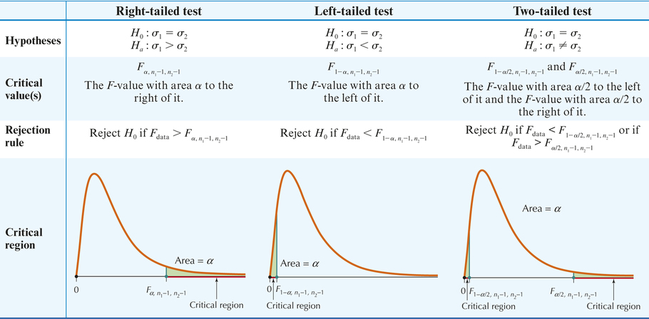
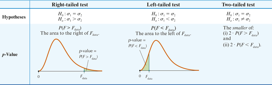
Table 16 provides the three possible forms of hypotheses available when performing the test for comparing two population standard deviations for two populations with standard deviations and , respectively.

618

Table 10.60: Table 16 Three possible forms for the test for comparing two population standard deviations

Form of test	Null hypothesis	Alternative hypothesis
Right-tailed test
Left-tailed test
Two-tailed test

The requirements for performing the test are the following:

We have two independent random samples taken from two populations.
The two populations are both normally distributed.

The test statistic for the test is , given as follows.

Test Statistic for the Test for Comparing Two Population Standard Deviations

Suppose that the two population variances are equal, , and that we have independent random samples of size and from two normally distributed populations with sample variances and , respectively. Then the test statistic for the test

follows an distribution with degrees of freedom in the numerator and degrees of freedom in the denominator.

Let's become better acquainted with the distribution. Similar to the distribution, the distribution is right-skewed, never takes negative values, and has an infinite number of different curves (Figure 20). The shape of the curve depends on degrees of freedom.

Figure 10.20: FIGURE 20 Shape of the distribution for various degrees of freedom.

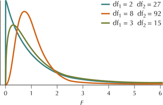
As noted, the distribution resembles the distribution. This is not surprising because the values of the distribution represent ratios of two distributions. Moreover, the distribution has two different degrees of freedom, which we will call and , derived from the degrees of freedom of the two distributions represented in the ratio. Often, is called the numerator degrees of freedom, and is called the denominator degrees of freedom.

Properties of the Curve

The total area under the curve equals 1.
The value of the random variable is never negative, so the curve starts at 0. However, it extends indefinitely to the right. The curve approaches but never quite meets the horizontal axis.
Because of the characteristics described in (2), the curve is right-skewed.
There is a different curve for each different pair of degrees of freedom: and .

619

The distribution is continuous, so we can find probabilities associated with values of , and vice versa, just as we did with the normal, , and distributions. Just as for any continuous distribution, probability is represented by the area below the curve above an interval.

2 Perform the Test for Comparing Two Population Standard Deviations: Critical-Value Method

To perform the hypothesis tests in this section, as well as in Chapters 12 and 13, we need to find the critical values of an distribution for a given level of significance . For example, we may need to find the value of an distribution that has area to the right of it, or we may need to find the value of an distribution that has area to the left of it. To find these critical values, we will work with the tables (see Appendix Table F). The tables are somewhat different from the other tables that we have worked with so far.

The notation

represents the critical value of the distribution with numerator degrees of freedom and denominator degrees of freedom, with area to the right of . For example, represents the value of the distribution with and , with area 0.05 to the right of it. Next, we learn how to find the critical values using the tables.

Procedure for Finding Critical Value for a Given Area to the Right of it

Suppose we have an distribution with and degrees of freedom. To find the critical value that has area to the right of it, do the following:

Step 1 Look across the top of the table until you find your . Then go down that column until you see your on the left.
Step 2 For each on the left, you will see a range of values from 0.100 to 0.001. Choose the row next to that has your value of . The -value in that row and column is your value of .

Note: When the degrees of freedom are not listed in the table, we do not necessarily take the closest degrees of freedom we can find. This is because, sometimes, the closest degree of freedom is larger than the original, which leads to misleadingly overprecise results—α level of precision not warranted by the data. For example, this could lead us to find significance where none actually exists.

Developing Your Statistical Sense

Degrees of Freedom Not Listed in the Table

Just as with the table, not all the degrees of freedom are listed in the table. If either of the degrees of freedom or are not listed in the table, a conservative solution is to take the next smallest value for whichever of or is not listed. For example, suppose and . Neither nor is given in the table. Therefore, we set df to be the next smallest value given in the table, , and we set to be the next smallest value, .

The tables give only the critical values for a given area to the right. To find critical values for a given area to the left, we use the following property:

In other words, the value from an distribution with degrees of freedom and and area to the left of it equals the reciprocal of the value from an distribution with degrees of freedom and and area to the right of it. Note that the two degrees of freedom get switched.

620

Procedure for Finding Critical Value for a Given Area to the Left of it

Switch the values of and .
Find using the table.
Calculate

So, for example, to find the value of an distribution with degrees of freedom and with area to the left of it, follow steps 1 and 2 above to find the value of an distribution with and with area to the right of it. Then compute the reciprocal.

EXAMPLE 19 Finding critical values of the distribution

Use the excerpt from the distribution tables in Figure 21 to find the following critical values of the distribution:

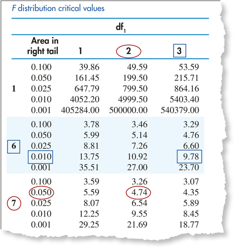
Figure 10.21: FIGURE 21 table (excerpt).

Find the critical value with area to the right of it, for an distribution with and .
Find the critical value with area to the left of it, for an distribution with and .

Solution

- Step 1. Go across the top of the table until we get to , and go down that column until we see on the left.
- Step 2. Next to the 7 is a range of values from 0.100 to 0.001. We choose the row with . The -value in that row and column is 4.74. Thus, our critical value is
  
  621
- Step 1. Switching the two degrees of freedom, we go across the top of the table until we get to . Then we go down that column until we see on the left.
- Step 2. Choose the row with . The -value in that row and column is 9.78. Thus, our critical value is

NOW YOU CAN DO

Exercises 9–20.

Now we use the critical values of the distribution to help us with the critical-value method of performing the test for comparing two population standard deviations. Later we show the steps for the -value method, along with an example.

Test for Comparing Two Population Standard Deviations: Critical-Value Method

Suppose we have two independent random samples of size and taken from two normally distributed populations, with population standard deviations and , and sample standard deviations and , respectively.

Step 1 State the hypotheses. Use one of the forms from Table 17. State the meaning of and .
Step 2 Find the critical value(s) and state the rejection rule. Use Table 17 and the tables.
Step 3 Find .

follows an distribution with and .
Step 4 State the conclusion and the interpretation. Compare with the critical value from Table 17.

Table 10.61: Table 17 Critical values, rejection rules, and rejection regions

622

We now return to our example comparing the variability of stock prices between Google and Apple.

EXAMPLE 20 test for comparing two population standard deviations: Critical-value method

Table 18 shows independent samples from Google and Apple stock prices from July 2014 together with the sample sizes and sample standard deviations. Test, using the critical-value method, whether the standard deviation of Google stock prices is greater than the standard deviation of Apple stock prices .

Table 10.62: Table 18 Independent random samples of stock prices, July 2014

Google	Apple
574.79 590.76 583.04 593.06 580.82 599.02 579.55 587.78	93.52 94.03 95.39 96.45 95.60 99.02 97.03

Table 10.62: Source: www.marketwatch.com/tools/quotes/historical.asp.

Solution

The normal probability plots in Figures 22a and 22b show acceptable normality for both samples. We may, therefore, proceed with the test for comparing population standard deviations.

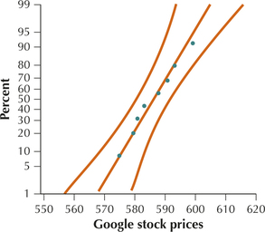
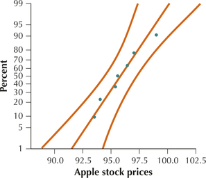
Figure 10.22: FIGURE 22a Normal probability plot of Google stock prices.

Figure 10.23: FIGURE 22b Normal probability plot of Apple stock prices.

Step 1 State the hypotheses. We are testing whether Google's stock prices are more variable than those of Apple. Thus, because Google represents population 1, we have the following hypotheses for our test:

where represents the standard deviation of Google stock prices and represents the standard deviation of Apple stock prices. Use level of significance .
Step 2 Find the critical value and state the rejection rule. We have and . From Table 17 and Appendix Table F, our critical value is the -value with area to the right of it:

Our rejection rule is, therefore, from Table 17: Reject if .

623
Step 3 Find

follows an distribution with and .
Step 4 State the conclusion and the interpretation. Because is greater than , we reject . There is evidence that the variability in Google stock prices is greater than the variability in Apple stock prices.

NOW YOU CAN DO

Exercises 21–26.

3 Perform the Test for Comparing Two Population Standard Deviations: -Value Method

We may also use the -value method to perform the test for comparing two population standard deviations. The requirements are the same.

Test for comparing two Population Standard Deviations: -Value Method

Suppose we have two independent random samples of size , and taken from two normally distributed populations, with population standard deviations and , and sample standard deviations and , respectively.

Step 1 State the hypotheses and the rejection rule. Use one of the forms from Table 19. Clearly state the meaning of and . The rejection rule is: Reject if the -value is less than .
Step 2 Find .

follows an distribution with and .
Step 3 Find the -value. Use technology and Table 19 to find the -value.
Step 4 State the conclusion and the interpretation. Compare the -value with .

Table 10.63: Table 19 -Value for the test for comparing two standard deviations

We illustrate the -value method with an example.

EXAMPLE 21 Test for comparing two population standard deviations: -value method

The Web site Medicare.gov publishes survey information on patient attitudes about their level of care. Table 20 shows the percentages of respondents taken from independent random samples of hospitals in Florida and Georgia, which reported that their nurses always communicated well.

624

Table 10.64: Table 20 Independent random samples of hospital percentages

Florida	Georgia
67 66 70 70 72 73	72 75 78 73 68 71
63 69 65 68 65	82 72 77 75 73

Table 10.64: Source: Medicare.gov.

Test whether there is a difference in variability between the two states, using .

Solution

Because the normal probability plots in Figures 23a and 23b show acceptable normality, we may therefore proceed with the test for comparing population standard deviations.

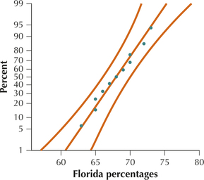
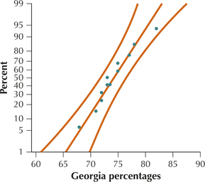
Figure 10.24: FIGURE 23a Normal probability plot of Florida percentages.

Figure 10.25: FIGURE 23b Normal probability plot of Georgia percentages.

Step 1 State the hypotheses. We are testing whether there is a difference in the standard deviation of the percentages for Florida () and Georgia (). We therefore have a two-tailed test:

where and represent the standard deviations of the percent of Florida and Georgia respondents, respectively, who reported that their nurses always communicated well. Use level of significance .
Step 2 Find .

follows an distribution with and .
Step 3 Find the -value. Because we have a two-tailed test, Table 19 states that the -value is

Figure 24a shows the output from the TI-83/84, giving as the area under the distribution curve between 0.6729 and infinity. This gives

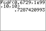Figure 10.26: FIGURE 24a

This cannot represent a valid -value, because it is larger than 1. Figure 24b shows the output from the TI-83/84, giving as the area under the distribution curve between 0 and 0.6729. Thus, our -value is:

because this is smaller than 1.457484199.

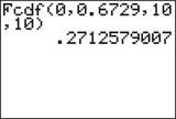Figure 10.27: FIGURE 24b

625
Step 4 State the conclusion and the interpretation. The -value 0.5425 is not less than , so we do not reject . There is insufficient evidence for a difference in population standard deviations between percentages of patients in Florida and Georgia hospitals who reported that their nurses always communicated well.

NOW YOU CAN DO

Exercises 27–32.