Section 13.1 Exercises
CLARIFYING THE CONCEPTS
Question 13.1
1. What is the difference between the regression equation (calculated using the sample) and the population regression equation? (p. 718)
13.1.1
The regression equation is calculated from a sample and is valid only for values of x in the range of the sample data. The population regression equation may be used to approximate the relationship between the predictor variable x and the response variable y for the entire population of (x, y) pairs.
Question 13.2
2. What are the four regression model assumptions? (p. 718)
Question 13.3
3. How do we go about verifying the regression model assumptions? (p. 719)
13.1.3
We construct a scatterplot of the residuals against the fitted values and a normal probability plot of the residuals. We must make sure that the scatterplot contains no strong evidence of any unhealthy patterns and that the normal probability plot indicates no evidence of departures from normality in residuals.
Question 13.4
4. What is the difference between b0 and b1 on the one hand and β0 and β1 on the other hand? (p. 718)
Question 13.5
5. What does it mean for the relationship between x and y when β1 equals 0? (p. 721)
13.1.5
There is no relationship between x and y.
Question 13.6
6. What is the difference between s and sx? (p. 722)
PRACTICING THE TECHNIQUES
 CHECK IT OUT!
| To do | Check out | Topic |
|---|---|---|
| Exercises 7–14 | Example 2 | Calculating the residuals and verifying the regression assumptions |
| Exercises 15–18 | Example 4 | Test for the slope β1: critical-value method |
| Exercises 19–22 | Example 5 | Test for the slope β1: p -value method |
| Exercises 23–30 | Example 6 | Confidence interval for the slope β1 |
| Exercises 31–38 | Example 7 | Using confidence intervals to perform the t test for the slope β1 |
For Exercises 7–14, you are given the regression equation.
- Calculate the predicted values.
- Compute the residuals.
- Construct a scatterplot of the residuals versus the predicted values.
- Use technology to construct a normal probability plot of the residuals.
- Verify that the regression assumptions are valid.
Question 13.7
7.
| x | y |
|---|---|
| 1 | 15 |
| 2 | 20 |
| 3 | 20 |
| 4 | 25 |
| 5 | 25 |
| ˆy = 2.5x + 13.5 | |
13.1.7
(a) and (b)
| x | y | Predicted value ˆy=13.5+2.5x |
Residual (y−ˆy) |
|---|---|---|---|
| 1 | 15 | 16 | –1 |
| 2 | 20 | 18.5 | 1.5 |
| 3 | 20 | 21 | –1 |
| 4 | 25 | 23.5 | 1.5 |
| 5 | 25 | 26 | –1 |
(c) and (d) See Solutions Manual. (e) The scatterplot of the residuals contains an unhealthy pattern, so the regression assumptions are not verified.
Question 13.8
8.
| x | y |
|---|---|
| 0 | 10 |
| 5 | 20 |
| 10 | 45 |
| 15 | 50 |
| 20 | 75 |
| ˆy = 3.2x + 8 | |
Question 13.9
9.
| x | y |
|---|---|
| −5 | 0 |
| −4 | 8 |
| −3 | 8 |
| −2 | 16 |
| −1 | 16 |
| ˆy = 4x + 21.6 | |
13.1.9
(a) and (b)
| x | y | Predicted value ˆy=21.6+4x |
Residual (y−ˆy) |
|---|---|---|---|
| –5 | 0 | 1.6 | –1.6 |
| –4 | 8 | 5.6 | 2.4 |
| –3 | 8 | 9.6 | –1.6 |
| –2 | 16 | 13.6 | 2.4 |
| –1 | 16 | 17.6 | –1.6 |
(c) and (d) See Solutions Manual. (e) The scatterplot of the residuals contains an unhealthy pattern, so the regression assumptions are not verified.
Question 13.10
10.
| x | y |
|---|---|
| −3 | −5 |
| −1 | −15 |
| 1 | −20 |
| 3 | −25 |
| 5 | −30 |
| ˆy =−3x − 16 | |
Question 13.11
11.
| x | y |
|---|---|
| 10 | 100 |
| 20 | 95 |
| 30 | 85 |
| 40 | 85 |
| 50 | 80 |
| ˆy = − 0.5x +104 | |
13.1.11
(a) and (b)
| x | y | Predicted value ˆy=104−0.5x |
Residual (y−ˆy) |
|---|---|---|---|
| 10 | 100 | 99 | 1 |
| 20 | 95 | 94 | 1 |
| 30 | 85 | 89 | –4 |
| 40 | 85 | 84 | 1 |
| 50 | 80 | 79 | 1 |
(c) and (d) See Solutions Manual. (e) The scatterplot of the residuals contains an unhealthy pattern, so the regression assumptions are not verified.
Question 13.12
12.
| x | y |
|---|---|
| 0 | 11 |
| 20 | 11 |
| 40 | 16 |
| 60 | 21 |
| 80 | 26 |
| ˆy = 0.2x + 9 | |
Question 13.13
13.
| x | y |
|---|---|
| 1 | 1 |
| 2 | 1 |
| 3 | 2 |
| 4 | 3 |
| 5 | 3 |
| ˆy =0.6x + 0.2 | |
13.1.13
(a) and (b)
| x | y | ˆy=0.6x+0.2 | y−ˆy |
|---|---|---|---|
| 1 | 1 | 0.8 | 0.2 |
| 2 | 1 | 1.4 | –0.4 |
| 3 | 2 | 2 | 0 |
| 4 | 3 | 2.6 | 0.4 |
| 5 | 3 | 3.2 | –0.2 |
(c)
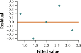
(d)
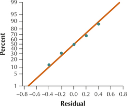
(e) The scatterplot in (c) of the residuals versus fitted values shows no strong evidence of unhealthy patterns. Thus, the independence assumption, the constant variance assumption, and the zero-mean assumption are verified. Also, the normal probability plot of the residuals in (d) indicates no evidence of departure from normality of the residuals. Therefore we conclude that the regression assumptions are verified.
Question 13.14
14.
| x | y |
|---|---|
| 1 | 6 |
| 2 | 5 |
| 2 | 4 |
| 2 | 3 |
| 3 | 2 |
| ˆy =−2x + 8 | |
For Exercises 15–18, follow these steps. Assume that the regression model assumptions are valid.
- Find tcrit for a two-tailed test with level of significance α=0.05 and df=n−2.
- Calculate s.
- Compute ∑(x − ˉx)2.
- Calculate tdata.
- Perform the hypothesis test for the linear relationship between x and y, using the critical-value method and α = 0.05.
Question 13.15
15. Data in Exercise 7, where b1 = 2.5
13.1.15
(a) tcrit=3.182 (b) s=1.58113883 (c) ∑(x−ˉx)2=10 (d) tdata=5 (e) H0:β1=0: There is no linear relationship between x and y. Ha:β1≠0: There is a linear relationship between x and y. Reject H0 if tdata≥3.182 or tdata≤−3.182. Since tdata=5≥3.182, we reject H0. There is evidence at level of significance α=0.05 that β1≠0 and that there is a linear relationship between x and y.
Question 13.16
16. Data in Exercise 8, where b1 = 3.2
Question 13.17
17. Data in Exercise 9, where b1 = 4.0
13.1.17
(a) tcrit=3.182 (b) s=2.529822128 (c) ∑(x−ˉx)2=10 (d) tdata=5 (e) H0:β1=0: There is no linear relationship between x and y. Ha:β1≠0: There is a linear relationship between x and y. Reject H0 if tdata≥−3.182 or tdata≤−3.182. Since tdata=5≥−3.182, we reject H0. There is evidence at level of significance α=0.05 that β1≠0 and that there is a linear relationship between x and y.
Question 13.18
18. Data in Exercise 10, where b1 = −3
For Exercises 19–22, follow these steps. Assume that the regression model assumptions are valid.
- Calculate s.
- Compute ∑(x − ˉx)2.
- Calculate tdata.
- Find p-valueP(t > | tdata |) .
- Perform the hypothesis test for the linear relationship between x and y using the p-value method and level of significance α = 0.05.
Question 13.19
19. Data in Exercise 11, where b1 = − 0.5
13.1.19
(a) s=2.581988897 (b) ∑(x−ˉx)2=100 (c) tdata=−6.1237 (d) p-value=0.0088 (e) H0:β1=0: There is no linear relationship between x and y. Ha:β1≠0: There is a linear relationship between x and y. Reject H0 if p-value ≤0.05. Since p-value =0.0088≤0.05, we reject H0. There is evidence at level of significance α=0.05 that β1≠0 and that there is a linear relationship between x and y.
Question 13.20
20. Data in Exercise 12, where b1 = 0.2
Question 13.21
21. Data in Exercise 13, where b1 = 0.6
13.1.21
(a) s=0.3651483717 (b) ∑(x−ˉx)2=10 (c) tdata=5.1962
(d) p-value=0.0138 (e) H0:β1=0: There is no linear relationship between x and y. Ha:β1≠0: There is a linear relationship between x and y. Reject H0 if p-value ≤0.05. Since p-value =0.0138≤0.05, we reject H0. There is evidence at level of significance α=0.05 that β1≠0 and that there is a linear relationship between x and y.
Question 13.22
22. Data in Exercise 14, where b1 = −2
For Exercises 23–30, follow these steps. Assume that the regression model assumptions are valid.
- Find tα/ 2 for a 95% confidence interval for β1.
- Find the margin of error E.
- Construct a 95% confidence interval for β1.
Question 13.23
23. Data in Exercise 7
13.1.23
(a) tα/2=3.182 (b) E=1.591 (c) (0.909, 4.091)
Question 13.24
24. Data in Exercise 8
Question 13.25
25. Data in Exercise 9
13.1.25
(a) tα/2=3.182 (b) E=2.5456 (c) (1.4544, 6.5456)
Question 13.26
26. Data in Exercise 10
Question 13.27
27. Data in Exercise 11
13.1.27
(a) tα/2=3.182 (b) E=0.2598 (c) (–0.7598, −0.2402)
Question 13.28
28. Data in Exercise 12
Question 13.29
29. Data in Exercise 13
13.1.29
(a) tα/2=3.182 (b) E=0.3674 (c) (0.2326, 0.9674). TI-83/84: (0.2325, 0.9675)
Question 13.30
30. Data in Exercise 14
For Exercises 31–38, using the confidence interval from the indicated exercise, perform the t test for β1 at level of significance α = 0.05.
Question 13.31
31. Exercise 23
13.1.31
H0:β1=0: There is no linear relationship between x and y. Ha:β1≠0: There is a linear relationship between x and y. Since the confidence interval from Exercise 23 (c) does not contain zero, we may conclude that β1≠0 and that a linear relationship exists between x and y, at level of significance α=0.05.
Question 13.32
32. Exercise 24
Question 13.33
33. Exercise 25
13.1.33
H0:β1=0: There is no linear relationship between x and y. Ha:β1≠0: There is a linear relationship between x and y. Since the confidence interval from Exercise 25 (c) does not contain zero, we may conclude that β1≠0 and that a linear relationship exists between x and y, at level of significance α=0.05.
Question 13.34
34. Exercise 26
Question 13.35
35. Exercise 27
13.1.35
H0:β1=0: There is no linear relationship between x and y. Ha:β1≠0 There is a linear relationship between x and y. Since the confidence interval from Exercise 27 (c) does not contain zero, we may conclude that β1≠0 and that a linear relationship exists between x and y, at level of significance α=0.05.
Question 13.36
36. Exercise 28
Question 13.37
37. Exercise 29
13.1.37
H0:β1=0: There is no linear relationship between x and y. Ha:β1≠0 There is a linear relationship between x and y. Since the confidence interval from Exercise 29 (c) does not contain zero, we may conclude that β1≠0 and that a linear relationship exists between x and y, at level of significance α=0.05.
Question 13.38
38. Exercise 30
APPLYING THE CONCEPTS
For Exercises 39–46, assume the regression requirements are met. Test for the linear relationship between x and y, using level of significance α = 0.05.
Question 13.39
volweight
39. Volume and Weight. The following table contains the volume (x, in cubic meters) and weight (y, in kilograms) of five randomly chosen packages shipped to a local college.
| Volume (x) |
Weight (y) |
|---|---|
| 4 | 10 |
| 8 | 16 |
| 12 | 25 |
| 16 | 30 |
| 20 | 35 |
13.1.39
H0:β1=0: There is no relationship between volume (x) and weight (y). Ha:β1≠0: There is a linear relationship between volume (x) and weight (y). Reject H0 if the p-value ≤ 0.05. Since the p-value ≈0.0006 is ≤0.05, we reject H0. There is evidence for a linear relationship between volume (x) and weight (y).
Question 13.40
familypet
40. Family Size and Pets. The number of family members (x) in a random sample taken from a suburban neighborhood, along with the number of pets (y) belonging to each family are shown in the following table.
| Family size (x) |
Pets (y) |
|---|---|
| 2 | 1 |
| 3 | 2 |
| 4 | 2 |
| 5 | 3 |
| 6 | 3 |
Question 13.41
worldtemp
41. World Temperatures. Listed in the following table are the low (x) and high (y) temperatures for a particular day, measured in degrees Fahrenheit, for a random sample of cities worldwide.
| City | Low (x) | High (y) |
|---|---|---|
| Kolkata | 57 | 77 |
| London | 36 | 45 |
| Montreal | 7 | 21 |
| Rome | 39 | 55 |
| San Juan | 70 | 83 |
| Shanghai | 34 | 45 |
13.1.41
H0:β1=0: There is no relationship between Low (x) and High (y).
Ha:β1≠0: There is a linear relationship between Low (x) and High (y).
Reject H0 if tdata≥2.776. Since tdata≈12.09 is ≥2.776, we reject H0. There is evidence for a linear relationship between Low (x) and High (y).
Question 13.42
videogamereg
42. Video Game Sales. The Chapter 1 Case Study looked at video game sales for the top 30 video games. The following table contains the total sales (y, in game units) and weeks on the top 30 list (x) of five randomly chosen video games.
| Video game | Weeks (x) | Total sales (y) |
|---|---|---|
| Super Mario Bros. U for WiiU | 78 | 1,690,689 |
| NBA 2K14 for PS4 | 27 | 608,899 |
| Battlefield 4 for PS3 | 29 | 911,687 |
| Titanfall for Xbox One | 10 | 1,150,856 |
| Yoshi's New Island for 3DS | 10 | 172,680 |
Question 13.43
dartsdjia
43. Darts and the Dow Jones. The following table contains a random sample of eight days from the Chapter 3 Case Study data set, indicating the stock market gain or loss for the portfolio chosen by the random darts (y), as well as the Dow Jones Industrial Average gain or loss for that day (x).
| Darts (y) | DJIA (x) |
|---|---|
| −27.4 | −12.8 |
| 18.7 | 9.3 |
| 42.2 | 8 |
| −16.3 | −8.5 |
| 11.2 | 15.8 |
| 28.5 | 10.6 |
| 1.8 | 11.5 |
| 16.9 | −5.3 |
13.1.43
H0:β1=0: No linear relationship exists between DJIA and darts.
Ha:β1≠0: A linear relationship exists between DJIA and darts.
Reject H0 if the p-value ≤α=0.05. tdata≈2.1749. p-value =0.0725703888.
The p-value=0.0725703888 is not ≤ α=0.05, so we do not reject H0. Insufficient evidence exists, at level of significance α=0.05, for a linear relationship between DJIA and darts.
Question 13.44
ageheight
44. Age and Height. The following table provides a random sample from the Chapter 4 Case Study data set Body Females, showing the age (x) and height (y) of the eight women.
| Age (x) | Height (y) |
|---|---|
| 40 | 63.5 |
| 28 | 63 |
| 25 | 64.4 |
| 34 | 63 |
| 26 | 63.8 |
| 21 | 68 |
| 19 | 61.8 |
| 24 | 69 |
Question 13.45
gardasilreg
45. Gardasil Shots and Age. The accompanying table shows a random sample of 10 patients from the Chapter 5 Case Study data set, Gardasil, including the age of the patient (x) and the number of shots taken by the patient (y).
| Age (x) | Shots (y) |
|---|---|
| 13 | 3 |
| 21 | 3 |
| 16 | 3 |
| 17 | 2 |
| 17 | 3 |
| 18 | 1 |
| 25 | 2 |
| 15 | 3 |
| 12 | 1 |
| 16 | 1 |
13.1.45
H0:β1=0: No linear relationship exists between age and shots.
Ha:β1≠0: A linear relationship exists between age and shots.
Reject H0 if the p-value ≤α=0.05. tdata≈0.1817. p-value=0.8603048707.
The p-value=0.8603048707 is not ≤α=0.05, so we do not reject H0. insufficient evidence exists, at level of significance α=0.05, for a linear relationship between a patient's age and the number of shots taken by the patient.
Question 13.46
ncaa2014
46. NCAA Power Ratings. The accompanying table shows the top 10 teams' winning percentage (x) and power rating (y) for the 2013-2014 NCAA basketball season, according to www.teamrankings.com.
| Team | Winning proportion (x) |
Power rating (y) |
|---|---|---|
| Florida | 0.923 | 121.2 |
| Wichita State | 0.971 | 119.1 |
| Arizona | 0.868 | 118.8 |
| Louisville | 0.838 | 117.9 |
| Connecticut | 0.800 | 117.2 |
| Virginia | 0.811 | 116.8 |
| Wisconsin | 0.789 | 116.6 |
| Villanova | 0.853 | 116.4 |
| Michigan State | 0.763 | 115.9 |
| Michigan | 0.757 | 115.9 |
For Exercises 47–54, do the following for the indicated data:
- Calculate the margin of error E for a 95% confidence interval for β1.
- Construct a 95% confidence interval for β1.
- Interpret the confidence interval.
Question 13.47
47. Volume and Weight. Data from Exercise 39.
13.1.47
(a) E=0.3312 (b) (1.2688, 1.9312) (c) We are 95% confident that the interval (1.2688, 1.9312) captures the population slope β1 of the relationship between volume and weight.
Question 13.48
48. Family Size and Pets. Data from Exercise 40
Question 13.49
49. World Temperatures. Data from Exercise 41
13.1.49
(a) E=0.2402 (b) (0.8064, 1.2868). TI-83/84: (0.8063, 1.2868) (c) We are 95% confident that the interval (0.8063, 1.2868) captures the population slope β1 of the relationship between Low and High.
Question 13.50
50. Video Game Sales. Data from Exercise 42
Question 13.51
51. Darts and the Dow Jones. Data from Exercise 43
13.1.51
(a) 1.5910 (b) (–0.1769, 3.0051) (c) We are 95% confident that the interval (–0.1769, 3.0051) captures the slope β1 of the population regression line. That is, we are 95% confident that for each additional $1 the stocks in the DJIA gain in one day, the daily change in the stocks in the portfolio predicted by the darts lies between –$0.039 and $0.66248.
Question 13.52
52. Age and Height. Data from Exercise 44
Question 13.53
53. Gardasil Shots and Age. Data from Exercise 45
13.1.53
(a) 0.19824 shot (b) (–0.1826, 0.21388) (c) We are 95% confident that the interval (–0.1826, 0.21388) captures the slope β1 of the population regression line. That is, we are 95% confident that for each additional year in a patient's age, the change in the number of shots taken by the patient lies between −0.1826 shot and 0.21388 shot.
Question 13.54
54. NCAA Power Ratings. Data from Exercise 46
Question 13.55
satfatreg
55. Saturated Fat and Calories. The table contains the calories and saturated fat in a sample of 10 food items.
- Construct a 90% confidence interval for the slope of the regression line, for the regression of calories on saturated fat.
- Using your confidence interval, conclude whether a linear relationship exists between calories and saturated fat, with level of significance α = 0.10.
| Food item | Calories | Grams of saturated fat |
|---|---|---|
| Chocolate bar (1.45 oz) | 215.66 | 6.9618 |
| Meat & veggie pizza, big slice (1/8 lg pizza) |
363.81 | 5.6472 |
| New England clam chowder (cup) |
148.80 | 1.8600 |
| Baked chicken drumstick (no skin, medium size) |
75.24 | 0.6424 |
| Curly fries, deep-fried (4 ounces) |
276.21 | 3.1752 |
| Wheat bagel (large) | 374.66 | 0.2751 |
| Chicken curry (cup) | 146.32 | 1.5930 |
| Cake doughnut hole (one) | 58.94 | 0.5068 |
| Rye bread (slice) | 67.34 | 0.1638 |
| Raisin Bran cereal (cup) | 194.59 | 0.3355 |
13.1.55
(a) (–6.647, 49.817) (b) 0 lies in the interval, so we do not reject H0.
Question 13.56
displacement
56. Engine Displacement and Gas Mileage. The table provides the engine displacement (size, in liters) and the city MPG (miles per gallon) gas mileage of a random sample of 12 vehicles.
- Construct a 95% confidence interval for the slope of the regression line, for the regression of city MPG on engine displacement.
- Using your confidence interval, conclude whether a linear relationship exists between city MPG and engine displacement, with level of significance α=0.05.
| Vehicle | Engine displacement |
City MPG |
|---|---|---|
| GMC Yukon Denali | 6.2 | 13 |
| Ford E350 Wagon | 5.4 | 11 |
| BMW 435i Coupe | 3.0 | 20 |
| Land Rover Range Rover | 5.0 | 13 |
| Infiniti Q50a | 3.7 | 19 |
| Dodge Journey | 3.6 | 17 |
| Jaguar XF | 5.0 | 15 |
| Dodge Challenger | 6.4 | 14 |
| Toyota Highlander Hybrid | 3.5 | 28 |
| Mercedes-Benz S 550 | 4.7 | 17 |
| Ford Fiesta | 1.6 | 29 |
| Hyundai Elantra | 2.0 | 24 |
Batting Average and Runs Scored. The table shows the top 10 hitters in Major League Baseball for 2013. We are interested in estimating the number of runs scored (y) by using the player's batting average (x). Use this information for Exercises 57–60.
| Batter | Team | Runs scored |
Batting average |
|---|---|---|---|
| Miguel Cabrera | Tigers | 103 | 0.348 |
| Mike Trout | Angels | 109 | 0.323 |
| Matt Carpenter | Cardinals | 126 | 0.318 |
| Andrew McCutchen | Pirates | 97 | 0.317 |
| Paul Goldschmidt | Diamondbacks | 103 | 0.302 |
| Josh Donaldson | Athletics | 89 | 0.301 |
| Chris Davis | Orioles | 103 | 0.286 |
| Carlos Gomez | Brewers | 80 | 0.284 |
| Manny Machado | Orioles | 88 | 0.283 |
| Evan Longoria | Rays | 91 | 0.269 |
Question 13.57
batters2013
57. Assess the regression assumptions. Is it okay to proceed with the regression?
13.1.57
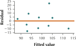
The scatterplot of the residuals versus the fitted values shows no evidence of the unhealthy patterns shown in Figure 4. Thus, the independence assumption, the constant variance assumption, and the zero-mean assumption are verified.
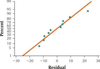
Also, the normal probability plot of the residuals indicates no evidence of departures from normality in the residuals. Therefore, we conclude that the regression assumptions are verified and it is okay to proceed with the regression.
Question 13.58
batters2013
58. Regress runs scored on batting average. Test for the significance of the linear relationship, using level of significance α= 0.10.
Question 13.59
batters2013
59. Find the residual for Matt Carpenter. What is unusual about Matt Carpenter in this regression?
13.1.59
22.51 runs; by far the highest number of runs scored but the third highest batting average.
Question 13.60
batters2013
60. Test for the significance of the linear relationship, using level of significance α = 0.05. Compare your conclusion with the earlier regression, using level of significance α = 0.05. How do you suggest we resolve this dilemma?
BRINGING IT ALL TOGETHER
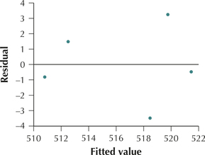
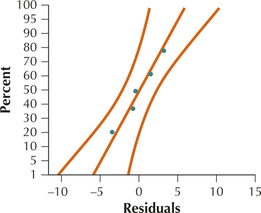
SAT Reading and Math Scores. Use this information for Exercises 61–65. The table shows the SAT scores for five states as reported by the College Board. We are interested in whether a linear relationship exists between the SAT Reading score (x) and the SAT Math score (y).
| State | SAT Reading (x) | SAT Math (y) |
|---|---|---|
| New York | 497 | 510 |
| Connecticut | 515 | 515 |
| Massachusetts | 518 | 523 |
| New Jersey | 501 | 514 |
| New Hampshire | 522 | 521 |
Question 13.61
statesat
61. What Result Might We Expect? Consider the accompanying scatterplot of Math score versus Reading score. Is there evidence for or against the null hypothesis that no linear relationship exists? Explain.
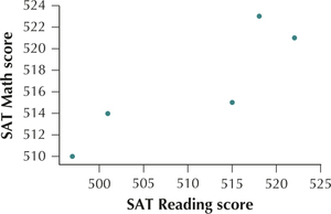
13.1.61
Against; the points appear to lie near a line with a positive slope.
Question 13.62
statesat
62. Consider the following graphics. Is there strong evidence that the regression assumptions are violated?
Question 13.63
statesat
63. Test, using level of significance α = 0.10, whether a linear relationship exists between the SAT reading score and the SAT Math score.
13.1.63
H0:β1=0: There is no linear relationship between SAT Reading score (x) and SAT Math score (y). Ha:β1≠0: There is a linear relationship between SAT Reading score (x) and SAT Math score (y). Reject H0 if tdata≥2.353 or tdata≤−2.353. Since tdata=3.1963≥−2.353, we reject H0. There is evidence at level of significance α=1.10 that β1≠0 and that there is a linear relationship between SAT Reading score (x) and SAT Math score (y).
Question 13.64
statesat
64. Construct and interpret a 90% confidence interval for a slope β1.
Question 13.65
statesat
65. Do your inferences in Exercises 63 and 64 agree with each other? Explain.
13.1.65
Yes. Since the confidence interval from Exercise 64 does not contain zero, we may conclude that β1≠0 and that a linear relationship exists between SAT Reading score (x) and SAT Math score (y), at level of significance α=0.10.
Question 13.66
 66. Challenge Exercise. Suppose we have a regression equation whose slope was not significant (that is, the null hypothesis was not rejected). What if we add five new data values to the original data set, and all five data values are identical, (ˉx,ˉy)? How and why will this affect the following statistics? Will the statistic increase, decrease, or remain unchanged, or is there insufficient information to determine? (Hint: The data point (ˉx,ˉy) always lies on the estimated regression line.)
- n
- SSR
- SST
- SSR
- MSE
- MSR
Question 13.67
67. Challenge Exercise. Refer to Exercise 66. How and why will the change affect the following items?
- tdata
- r2
- s
- p−value
- conclusion
13.1.67
(a) tdata increases if b1 is positive and decreases if b1 is negative. (b) r2 remains the same. (c) s decreases. (d) p-value decreases. (e) Since we don't know what the new p-value will be, we don't know if the p-value will decrease enough to change the conclusion from “Do not reject H0” to “Reject H0.”
Question 13.68
68. Challenge Exercise. Suppose a regression analysis of y on x was found to be significant (that is, the null hypothesis was rejected). What if we get 10 new data values, all with different values of x and all of which can be found on the estimated regression line of the original model? How and why will this change affect the following statistics? Will the statistic increase, decrease, or remain unchanged, or is there insufficient information to determine?
- n
- SSE
- SST
- SSR
- MSE
- MSR
Question 13.69
69. Refer to Exercise 68. How and why will this change affect the following measures?
- tdata
- r2
- s
- p−value
- conclusion
13.1.69
(a) tdata increases if b1 is positive and decreases if b1 is negative.
(b) r2 increases. (c) s decreases. (d) p-value decreases. (e) Unchanged.
Question 13.70
70. Challenge Exercise. Suppose a regression analysis of y on x was found to be significant (that is, the null hypothesis was rejected) and the slope b1> 0. Consider the observation (max , which represents the data value for the maximum value of in the data set. Suppose the residual for is negative. What if we increase max by an arbitrary amount so that the new data value is ? (All other data values in the data set are unchanged.) How will this increase affect the following measures? Will they increase, decrease, or remain unchanged, or is there insufficient information to determine the effect?
- SSE
- SST
- SSR
- MSE
- MSR
Question 13.71
71. Challenge Exercise. Refer to Exercise 70. How and why will the change affect the following measures?
- conclusion
13.1.71
(a-b) Decrease (c-d) Increase (e) Depends on the new -value.
WORKING WITH LARGE DATA SETS
For Exercises 72–74, use technology to solve the following problems:
- Verify the regression model assumptions.
- Construct and interpret a 95% confidence interval for .
- Based on the confidence interval constructed in (b), would you expect the hypothesis test to reject the null hypothesis that ?
- Test, at , whether a linear relationship exists between and .
Question 13.72
darts
72. Open the Darts data set, which we used for the Chapter 3 Case Study. Use the Dow Jones Industrial Average to estimate the pros' performance .
Question 13.73
nutrition
73. Open the Nutrition data set. Estimate the number of calories per gram using the amount of fat per gram .
13.1.73
(a) The scatterplot of the residuals contains evidence of an unhealthy pattern and the normal probability plot indicates evidence of departures from normality in the residuals. Therefore we conclude that the regression assumptions are not verified. (b) (7.821, 8.437). We are 95% confident that the interval (13.5483, 14.6201) captures the population slope of the relationship between fat per gram and calories per gram. (c) Yes (d) . There is no relationship between fat per gram () and calories per gram . There is a linear relationship between fat per gram () and calories per gram (). Reject if . -value ≈ 0. Since the , we reject . There is evidence for a linear relationship between fat per gram () and calories per gram ().
Question 13.74
pulseandtemp
74. Open the Pulse and Temp data set. Estimate body temperature using heart rate .
Use technology for Exercises 75–78. Open the Crash data set, which contains information about the severity of injuries sustained by crash dummies when the National Transportation Safety Board crashed automobiles into a wall at 35 miles per hour.
Question 13.75
crash
75. The variable head_inj contains a measure of the severity of the head injury sustained by the dummies. The variable chest_in is a measure of the severity of the chest injury suffered by the crash dummies.
- Would you expect a linear relationship to exist between the severity of head injuries and chest injuries?
- Construct a scatterplot of the head_inj against chest_in. Describe the relationship between the variables.
- If we were to perform a regression analysis using these two variables, is it clear which of the two variables we should label as the predictor and which we should label as the response? Explain.
13.1.75
(a) No (b) Positive relationship (c) Unclear
Question 13.76
crash
76. Perform a regression of the head injury severity on the chest injury severity .
- What is the regression equation? Write it out in words and numbers, so that a nonstatistician would understand it.
- Perform the appropriate hypothesis test, using level of significance .
- Clearly interpret the meaning of the slope estimate .
- Construct and interpret a 99% confidence interval for the true slope of the relationship between severity of head injury and severity of chest injury. How does your confidence interval support your conclusion in (b)?
Question 13.77
crash
77. The variable lleg_inj contains a measure of the severity of the injury sustained by the dummies' left legs. The variable weight contains the weight of the vehicles.
- Would you expect a linear relationship to exist between the severity of left leg injuries and the weight of the vehicles?
- Construct a scatterplot of the lleg_inj against weight. Describe the relationship between the variables.
- If we were to perform a regression analysis using these two variables, is it clear which of the two variables we should label as the predictor and which we should label as the response? Explain.
13.1.77
(a) No (b) No apparent relationship between the variables (c) The weight of vehicles is the predictor variable and the severity of the leg injuries should be the response variable.
Question 13.78
crash
78. Perform a regression of the left leg injury severity on the vehicle weight .
- What is the regression equation? Write it out in words and numbers, so that a nonstatistician would understand it.
- Is the relationship significant? Perform the appropriate hypothesis test, using level of significance .
- Construct and interpret a 95% confidence interval for the true slope of the relationship between vehicle weight and severity of left leg injury. How does your confidence interval support your conclusion in (b)?