Section 3.3 Exercises
CLARIFYING THE CONCEPTS
Question 3.214
1. Explain why the formula for the mean of grouped data will provide an estimate only and not the exact value of the mean if the data were not grouped. (p. 149)
3.3.1
These formulas will provide only estimates because we will not know the exact data values.
Question 3.215
2. Describe how the weighted mean is calculated. (p. 149)
Question 3.216
3. Suppose we calculate the weighted mean of the following data: 2, 7, 4. Let each of the weights equal 1. To what measure of center from Section 3.1 does this weighted mean simplify when all the weights equal 1? (p. 149)
3.3.3
The mean
PRACTICING THE TECHNIQUES
 CHECK IT OUT!
| To do | Check out | Topic |
|---|---|---|
| Exercises 4–8 | Example 17 | Weighted mean |
| Exercises 9–14 | Example 18 | Estimated mean for grouped data |
| Exercises 15–20 | Example 19 | Estimated variance and standard deviation for grouped data |
For Exercises 4–8, the data values and weights are provided. Find the weighted mean.
Question 3.217
4. x1=60, x2=70; x3=80; w1=0.25, w2=0.50, w3=0.25.
Question 3.218
5. x1=100, x2=60, x3=90; w1=0.25, w2=0.40, w3=0.35.
3.3.5
80.5
Question 3.219
6. x1=10, x2=10, x3=100; w1=10, w2=20, w3=5.
Question 3.220
7. x1=2.0, x2=3.5, x3=2.5, x4=3.0, x5=2.0; w1=w2=w3=w4=3, w5=8.
3.3.7
2.45
Question 3.221
8. x1=70, x2=80, x3=85, x4=95; w1=0.25, w2=0.25, w3=0.25, w4=0.25.
For Exercises 9–14, the frequency distribution is provided for a particular variable. Do the following:
- Find the class midpoints.
- Calculate the product of each class frequency with its midpoint.
- Find the sum of the frequencies, ∑f, and the sum of the products ∑(f·x).
- Divide ∑(f·x) by ∑f to find the estimated mean of the variable, ˉx.
Question 3.222
9.
| Class | Frequency f |
|---|---|
| 0≤GPA<1.0 | 2 |
| 1.0≤GPA<2.0 | 10 |
| 2.0≤GPA<3.0 | 13 |
| 3.0≤GPA<4.0 | 5 |
3.3.9
(a)-(c)
| Class | Frequency f | Midpoint x | Product f · x |
|---|---|---|---|
| 0≤GPA<1.0 | 2 | 0.5 | 1.0 |
| 1.0≤GPA<2.0 | 10 | 1.5 | 15.0 |
| 2.0≤GPA<3.0 | 13 | 2.5 | 32.5 |
| 3.0≤GPA<4.0 | 5 | 3.5 | 17.5 |
| Total | ∑f=30 | ∑(f⋅x)=66 |
(d) ˉx=∑(f⋅x)∑f=6630=2.2
Question 3.223
10.
| Class | Frequency f |
|---|---|
| -10≤golf score<−5 | 3 |
| -5≤golf score<0 | 7 |
| 0≤golf score<5 | 7 |
| 5≤golf score<10 | 3 |
Question 3.224
11.
| Class | Frequency f |
|---|---|
| 0≤score<2 | 10 |
| 2≤score<4 | 20 |
| 4≤score<6 | 30 |
| 6≤score<8 | 20 |
| 8≤score<10 | 10 |
3.3.11
(a)–(c)
| Class | Frequency f | Midpoint x | Product f · x |
|---|---|---|---|
| 0≤score<2 | 10 | 1 | 10 |
| 2≤score<4 | 20 | 3 | 60 |
| 4≤score<6 | 30 | 5 | 150 |
| 6≤score<8 | 20 | 7 | 140 |
| 8≤score<10 | 10 | 9 | 90 |
| Total | ∑f=90 | ∑(f⋅x)=450 |
(d) ˉx=∑(f⋅x)∑f=45090=5
Question 3.225
12.
| Class | Frequency f |
|---|---|
| 0≤grade<50 | 5 |
| 50≤grade<70 | 10 |
| 70≤grade<80 | 15 |
| 80≤grade<90 | 20 |
| 90≤grade<100 | 20 |
Question 3.226
13.
| Class | Frequency f |
|---|---|
| 0≤cost<5 | 100 |
| 5≤cost<10 | 150 |
| 10≤cost<15 | 200 |
| 15≤cost<20 | 250 |
| 20≤cost<30 | 300 |
| 30≤cost<50 | 350 |
| 50≤cost<100 | 400 |
| 100≤cost<200 | 450 |
3.3.13
(a)–(c)
| Class | Frequency f | Midpoint x | Product f⋅x |
|---|---|---|---|
| 0≤cost<5 | 100 | 2.5 | 250 |
| 5≤cost<10 | 150 | 7.5 | 1,125 |
| 10≤cost<15 | 200 | 12.5 | 2,500 |
| 15≤cost<20 | 250 | 17.5 | 4,375 |
| 20≤cost<30 | 300 | 25 | 7,500 |
| 30≤cost<50 | 350 | 40 | 14,000 |
| 50≤cost<100 | 400 | 75 | 30,000 |
| 100≤cost<200 | 450 | 150 | 67,500 |
| Total | ∑f=2200 | ∑(f⋅x)=127,250 |
(d) ˉx=∑(f⋅x)∑f=127,2502200=57.84
Question 3.227
14.
| Class | Frequency f |
|---|---|
| 0≤cash<10 | 15 |
| 10≤cash<20 | 10 |
| 20≤cash<30 | 5 |
| 30≤cash<40 | 4 |
| 40≤cash<50 | 4 |
| 50≤cash<75 | 2 |
| 75≤cash<100 | 1 |
| 100≤cash<200 | 1 |
For Exercises 15–20, find the estimated variance and standard deviation for the frequency distribution given in the indicated Exercise.
Question 3.228
15. Exercise 9.
3.3.15
Variance: s2=0.6767; Standard deviation: s=0.8226
Question 3.229
16. Exercise 10.
Question 3.230
17. Exercise 11.
3.3.17
Variance: s2=5.3333; Standard deviation: s=2.3094
Question 3.231
18. Exercise 12.
Question 3.232
19. Exercise 13.
3.3.19
Variance: s2=2672.3270; Standard deviation: s=51.6946
Question 3.233
20. Exercise 14.
APPLYING THE CONCEPTS
Question 3.234
dupageage
21. Dupage County age groups. The Census Bureau reports the following frequency distribution of population by age group for Dupage County, Illinois, for residents who are less than 65 years old.
| Class | Residents |
|---|---|
| 0≤age<5 | 63,422 |
| 5≤age<18 | 240,629 |
| 18≤age<65 | 540,949 |
- Find the class midpoints.
- Find the estimated mean age of residents of Dupage County.
- Find the estimated variance and standard deviation of ages.
3.3.21
(a)
| Age | Frequency | Midpoints |
|---|---|---|
| 0–4.99 | 63,422 | 2.5 |
| 5–17.99 | 240,629 | 11.5 |
| 18–64.99 | 540,949 | 41.5 |
(b) Estimated mean = 30.0298 years (c) Estimated standard deviation = 15.455909 years; estimated variance = 238.8851 years squared
Question 3.235
browardhouse
22. Broward County House Values. Table 19 gives the frequency distribution of the dollar value of the owner-occupied housing units in Broward County, Florida.
| Class (1000s) | Housing units |
|---|---|
| 0≤value<50 | 5,430 |
| 50≤value<100 | 90,605 |
| 100≤value<150 | 90,620 |
| 150≤value<200 | 54,295 |
| 200≤value<300 | 34,835 |
| 300≤value<500 | 15,770 |
| 500≤value<1000 | 5,595 |
- Find the class midpoints.
- Find the estimated mean dollar value for housing units in Broward County.
- Find the estimated variance and standard deviation of the dollar value.
Question 3.236
lightningdeath
23. Lightning Deaths. Table 20 gives the frequency distribution of the number of deaths due to lightning nationwide over a 67-year period. Find the estimated mean and standard deviation of the number of lightning deaths per year.
| Class | Years |
|---|---|
| 20≤deaths<60 | 13 |
| 60≤deaths<100 | 21 |
| 100≤deaths<140 | 10 |
| 140≤deaths<180 | 6 |
| 180≤deaths<260 | 10 |
| 260≤deaths<460 | 7 |
3.3.23
Estimated mean = 135.5224; estimated standard deviation = 95.6874
Question 3.237
24. Calculating a Course Grade. An introductory statistics syllabus has the following grading system. The weekly quizzes are worth a total of 25% toward the final course grade. The midterm exam is worth 32%; the final exam is worth 33%; and attendance/participation is worth 10% toward the final course grade. Anthony's weekly quiz average is 70. He got an 80 on the midterm and a 90 on the final exam. He got a 100 for attendance/participation. Calculate Anthony's final course grade.
Question 3.238
compwage
25. Wages for Computer Managers. The U.S. Bureau of Labor Statistics (BLS) publishes wage information for various occupations. For the occupation “computer and information systems management,” Table 21 gives the wages reported by the BLS for the top-paying states. Find the weighted mean wage across all five states, using the employment figures as weights.
| State | Employment | Hourly mean wage |
|---|---|---|
| New Jersey | 12,380 | $60.32 |
| New York | 18,580 | $60.25 |
| Virginia | 9,540 | $59.39 |
| California | 35,550 | $57.98 |
| Massachusetts | 10,130 | $55.95 |
3.3.25
$58.72
Question 3.239
26. Salaries of Scientists and Engineers. The National Science Foundation compiles statistics on the annual salaries of full-time employed doctoral scientists and engineers in universities and four-year colleges. The mean annual salary for the fields of science, engineering, and health are $67,000, $82,200, and $70,000, respectively. Suppose we have a sample of 10 professors, 5 of whom are in science, 2 in engineering, and 3 in health, and each of whom is making the mean salary for his or her field. Find the weighted mean salary of these 10 professors.
Question 3.240
27. Challenge Exercise. Assign the weights, w, to show that the formula for the sample mean from Section 3.1, ˉx=∑x/n, is a special case of the formula for the weighted mean, ˉx=∑(wx)/∑w.
3.3.27
If wi = 1 for all i, then the weighted mean formula will be equivalent to the formula for the sample mean.
BRINGING IT ALL TOGETHER
Wait Times at Los Angeles Airport. Use the following table for Exercises 28–33. The data represent the number of passengers whose flights were delayed at the Tom Bradley Terminal of Los Angeles Airport (LAX), on July 2, 2014, between 4 P.M. and 5 P.M. Counts are given based on how long their flights were delayed.
| Delay (minutes) | Passengers |
|---|---|
| 0 to<16 | 665 |
| 16 to<31 | 551 |
| 31 to<46 | 497 |
| 46 to<61 | 399 |
| 61 to<91 | 355 |
| 91 to<120 | 27 |
Question 3.241
28. Find the delay midpoints.
Question 3.242
29. Construct a table similar to Table 17, showing the frequencies, f, the midpoints, x, the products, f·x, the sum of the frequencies, ∑f, and the sum of the products, ∑(f·x).
3.3.29
| Delay (minutes) | Frequency f | Midpoint x | Product f⋅x |
|---|---|---|---|
| 0 to < 16 | 665 | 8 | 5,320 |
| 16 to < 31 | 551 | 23.5 | 12,948.5 |
| 31 to < 46 | 497 | 38.5 | 19,134.5 |
| 46 to < 61 | 399 | 53.5 | 21,346.5 |
| 61 to < 91 | 355 | 76 | 26,980 |
| 91 to < 120 | 27 | 105.5 | 2,848.5 |
| Total | ∑f=2494 | ∑(f⋅x)=88,578 |
Question 3.243
30. Use the quantities from Exercise 29 to calculate the estimated mean delay time.
Question 3.244
31. Extend your table from Exercise 29 so that it is similar to Table 18, including columns for ˉx, x-ˉx, and (x-ˉx)2·f. Calculate ∑(x-ˉx)2·f.
3.3.31
| Delay (minutes) | Midpoint x | Frequency f | ˉx | x−ˉx | (x−ˉx)2⋅f |
|---|---|---|---|---|---|
| 0 to < 16 | 8 | 665 | 35.52 | –27.52 | 503,638.016 |
| 16 to < 31 | 23.5 | 551 | 35.52 | –12.02 | 79,608.7004 |
| 31 to < 46 | 38.5 | 497 | 35.52 | 2.98 | 4,413.5588 |
| 46 to < 61 | 53.5 | 399 | 35.52 | 17.98 | 128,988.8796 |
| 61 to < 91 | 76 | 355 | 35.52 | 40.48 | 581,713.792 |
| 91 to < 120 | 105.5 | 27 | 35.52 | 69.98 | 132,224.4108 |
| Total | ∑f=2494 | ∑(x−x)2⋅f=1,430,587.3576 |
Question 3.245
32. Use the statistics from Exercise 31 to compute the estimated variance.
Question 3.246
33. Calculate the estimated standard deviation of delay times.
3.3.33
23.9502
WORKING WITH LARGE DATA SETS
 Financial Experts versus the Darts. This set of exercises examines how close the estimated mean, variance, and standard deviation are to their true values. Use the Darts data set from the Chapter 3 Case Study for Exercises 34–37.
Question 3.247
darts
34. Use the following classes to construct a frequency distribution for the professionals, Darts, and the DJIA data sets.
| Class |
|---|
| -50≤ price change <−25 |
| -25≤ price change <0 |
| 0≤ price change <25 |
| 25≤ price change <50 |
| 50≤ price change <75 |
| 75≤ price change <100 |
Question 3.248
darts
35. Use the frequency distribution from Exercise 34 to calculate the estimated mean stock price change for the professionals, Darts, and the DJIA data sets.
3.3.35
Professionals: 13.25
Darts: 5.5
DJIA: 7.75
Question 3.249
darts
36. Use the information from the two previous exercises to compute the estimated variance and standard deviation for the stock price changes for the professionals, Darts, and the DJIA data sets.
Question 3.250
darts
37. Using technology, find the mean, variance, and standard deviation for the professionals, Darts, and the DJIA data sets. Calculate the difference between the estimated values and the actual values.
3.3.37
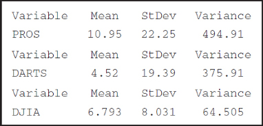
Professionals:
Mean: 10.95 10.95−13.25=−2.3
Variance: 494.91−555.69=−6078
Standard deviation: 22.25−23.57=−1.32
Darts:
Mean: 4.52−5.5=−0.98
Variance: 375.91−376=−0.09
Standard deviation: 19.39−19.39=0
DJIA:
Mean: 6.793−7.75=−0.957
Variance: 64.505−96.188=−31.683
Standard deviation: 8.031−9.808=−1.777
WORKING WITH LARGE DATA SETS
Year-by-year age distribution. Open the Age Distribution 100 data set, and use it for Exercises 38–42. This data set shows the year-by-year age distribution of Americans under age 100, as reported by the U.S. Census Bureau, for 2011. Use technology to answer the following:
Question 3.251
agedistribution100
38. How many tiny tots have yet to reach their first birthday?
Question 3.252
agedistribution100
39. Find the mean age of Americans under 100.
3.3.39
37.30 years
Question 3.253
agedistribution100
40. Calculate the estimated standard deviation of Americans under 100.
Question 3.254
agedistribution100
41. Use the Empirical Rule (see Section 3.2) to find two age values between which lie about 68% of the ages of all Americans under 100.
3.3.41
14.6 years and 60 years
Question 3.255
agedistribution100
42. Compute the actual proportion between the age values found in the previous exercise. Compare the actual number to the estimate in the previous exercise.