3.2 Measures of Variability
OBJECTIVES By the end of this section, I will be able to …
- Find the range of a data set.
- Calculate the variance and the standard deviation for a population.
- Compute the variance and the standard deviation for a sample.
- Use the Empirical Rule to find approximate percentages for a bell-shaped distribution.
- Apply Chebyshev's Rule to find minimum percentages.
1 The range
In Section 3.1, we learned how to find the center of a data set. Is that all there is to know about a data set? Defnitely not! Two data sets can have exactly the same mean, median, and mode and yet be quite different. We need measures that summarize the data set in a different way, namely, the variation or variability of the data. In Section 3.2, we will learn measures of variability that will help us answer the question: “How spread out is the data set?”
EXAMPLE 8 Different data sets with the same measures of center

Table 10 contains the heights (in inches) of the players on two volleyball teams.
| Western Massachusetts University |
Northern Connecticut University |
|---|---|
| 60 | 66 |
| 70 | 67 |
| 70 | 70 |
| 70 | 70 |
| 75 | 72 |
volleyball
- Describe in words and graphs the variability of the heights of the two teams.
- Verify that the means, medians, and modes for the two teams are equal.
Solution
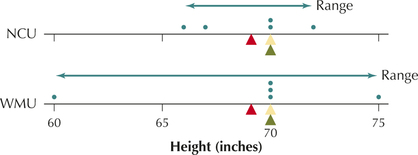
- There are some distinct differences between the teams. The Western Massachusetts (WMU) team has a player who is relatively short (60 inches: 5 feet tall) and a player who is very tall (75 inches: 6 feet, 3 inches tall). The Northern Connecticut (NCU) team has players whose heights are all within 6 inches of each other.
- But despite the differences in (a), the mean, median, and mode of the heights for the two teams are precisely the same. As illustrated in Figure 11, the mean height (red triangle) for each team is 69 inches, the median height (green triangle) for each team is 70 inches, and the mode height (yellow triangle) for each team is 70 inches.
ˉxWMU=60+70+70+70+755=3455=69ˉxNCU=66+67+70+70+725=3455=69
Clearly, these measures of location do not give us the whole picture. We need measures of variability (or measures of spread or measures of dispersion) that will describe how spread out the data values are. Figure 11 illustrates that the heights of the WMU team are more spread out than the heights of the NCU team.
Just as there were several measures of the center of a data set, there are also a variety of ways to measure how spread out a data set is. The simplest measure of variability is the range.
The range of a data set is the difference between the largest value and the smallest value in the data set:
range=largest value-smallest value=maximum-minimun
A larger range is an indication of greater variability, or greater spread, in the data set.
EXAMPLE 9 Range of the volleyball teams' heights
Calculate the range of player heights for each of the WMU and NCU teams.
Solution
What Results Might We Expect?
From Figure 11, it is intuitively clear that the heights of the WMU team are more spread out than the heights of the NCU team. Therefore, we would expect the range of the WMU team to be larger than the range of the NCU team, reflecting its greater variability.
rangeWMU=largest value-smallest value=75-60=15 inchesrangeNCU=largest value-smallest value=72-66=6 inches
As we expected, the range for WMU players is indeed larger than the range for NCU players, refecting WMU's players' greater variability in height.
NOW YOU CAN DO
Exercises 11a–16a.
YOUR TURN#4
 Table 11 contains a sample from the data set for the Chapter 3 Case Study. The percent increase or decrease in stock portfolio is recorded for the set of stocks chosen by throwing darts at the stock pages, along with the Dow Jones Industrial Average (DJIA) for the same day.
| Darts | DJIA |
|---|---|
| 11.2 | 15.8 |
| 72.9 | 16.2 |
| 16.6 | 17.3 |
| 28.7 | 17.7 |
- Construct a comparison dotplot of the darts returns and the DJIA returns.
- Using the dotplot, which group would you say has the larger range?
- Calculate the range for each group. Is your intuition from (2) confirmed?
(The solutions are shown in Appendix A.)
The range is quite simple to calculate; however, it does have its drawbacks. For example, the range is quite sensitive to extreme values, because it is calculated from the difference of the two most extreme values in the data set. It completely ignores all the other data values in the data set. We would prefer our measure of variability to quantify spread with respect to the center, as well as to actually use all the available data values. Two such measures are the variance and the standard deviation.
2 Population Variance and Population Standard Deviation
Before we learn about the variance and the standard deviation, we need to get a firm understanding of what a deviation means, in the statistical sense.
Deviation
A deviation for a given data value x is the difference between the data value and the mean of the data set. For a sample, the deviation equals x-ˉx. For a population, the deviation equals x-μ.
- If the data value is larger than the mean, the deviation will be positive.
- If the data value is smaller than the mean, the deviation will be negative.
- If the data value equals the mean, the deviation will be zero.
The deviation can roughly be thought of as the distance between a data value and the mean, except that the deviation can be negative, whereas distance is always positive.
EXAMPLE 10 Calculating deviations

Ashley and Brandon are certified public accountants who work for a large accounting firm, preparing tax returns for small business clients. Because tax returns are often fled close to the deadline, it is important that the returns be prepared in a timely fashion, with not a lot of variability in the length of time it takes to prepare a return. The chief accountant kept careful track of the amount of time (in hours, Table 12) for all the tax returns prepared by Ashley and Brandon during the last week of March.
- Find the mean preparation time for each accountant.
- Use comparative dotplots to compare the variability of Ashley and Brandon's tax preparation times.
- Calculate the deviations for each of Ashley and Brandon's tax preparation times.
| Ashley | 5 | 7 | 8 | 9 | 11 |
| Brandon | 3 | 5 | 7 | 11 | 14 |
Solution
Because the data represent all the tax returns for the indicated period, they may be considered a population.
- For Ashley:
μ=∑xN=5+7+8+9+115=8 hours
For Brandon:
μ=∑xN=3+5+7+11+145=8 hours
So the two accountants spent the same mean amount of time in tax preparation.
Figure 12 contains comparative dotplots of Ashley and Brandon's tax preparation times. Note that Brandon's preparation times vary more than Ashley's. Compared to Ashley, we can say that Brandon's tax preparation times
- are more spread out,
- show greater variability,
- have more variation, and
- are more dispersed.
The chief accountant probably prefers a more consistent tax preparation time, with less variability.
 FIGURE 12 Brandon's tax preparation times are more spread out.Page 130
Here we find the deviations, x-μ.
- Ashley's mean preparation time is μ=8 hours. Her first tax return took x=5 hours, so the deviation for this first tax return is x-μ=5-8=−3. Note that, when x<μ, the deviation is negative.
- Ashley's last tax return took 11 hours, so the deviation for this last return is x-μ=11-8=3. Note that, x>μ, the deviation is positive.
- Continuing in this way, we find the deviations for all of Ashley's and Brandon's tax preparation times, as recorded in Table 13.
| Ashley's times | 5 | 7 | 8 | 9 | 11 |
| Ashley's deviations | 5-8=−3 | 7-8=−1 | 8-8=0 | 9-8=1 | 11-8=3 |
| Brandon's times | 3 | 5 | 7 | 11 | 14 |
| Brandon's deviations | 3-8=−5 | 5-8=−3 | 7-8=−1 | 11-8=3 | 14-8=6 |
NOW YOU CAN DO
Exercises 11c–16c.
These deviations are used for the most widespread measures of spread: the variance and the standard deviation. However, we cannot use the mean deviation, because the mean deviation always equals zero. For example,
- Ashley's mean deviation: (-3)+(-1)+0+1+35=0
- Brandon's mean deviation: (-5)+(-3)+(-1)+3+65=0
The mean deviation always equals zero for any data set because the positive and negative deviations cancel each other out. Thus, the mean deviation is not a useful measure of spread. To avoid this problem, we will work with the squared deviations.
Table 14 shows the squared deviations for Ashley and Brandon. Note that Brandon's squared deviations are, on average, larger than Ashley's, reflecting the greater spread in Brandon's preparation times. It is therefore logical to build our measure of spread using the mean squared deviation.
| Ashley's deviations | −3 | −1 | 0 | 1 | 3 |
| Ashley's squared deviations | 9 | 1 | 0 | 1 | 9 |
| Brandon's deviations | −5 | −3 | −1 | 3 | 6 |
| Brandon's squared deviations | 25 | 9 | 1 | 9 | 36 |
The Population Variance, σ2
For populations, the mean squared deviation is called the population variance and is symbolized by σ2. This is the lowercase Greek letter sigma, not to be confused with the uppercase sigma (∑) used for summation.
The population variance, σ2, is the mean of the squared deviations in the population and is given by the formula
σ2=∑(x -
Notice that the numerator in is a sum of squares. Squared numbers can never be negative, so a sum of squares also can never be negative. The denominator, , which is the population size, also can never be negative. Thus, can never be negative. The only time is when all the population data values are equal.
EXAMPLE 11 Calculating the population variances for Ashley and Brandon
Calculate the population variances of the tax preparation times for Ashley and Brandon.
Solution
Using the squared deviations from Table 14, we have
for Ashley, and
for Brandon. The population variance of the tax preparation times for Brandon is greater than the variance for Ashley, thus indicating that Brandon's tax preparation times are more variable than Ashley's.
NOW YOU CAN DO
Exercises 11d–16d.
YOUR TURN#5
Table 15 contains the funding provided by the Centers for Disease Control (CDC) to all the states in New England, in order to fight HIV/AIDS.3 This includes all the states in New England, so we may consider this a population.
- Find the population mean funding, .
- Calculate the population variance of the funding, .
(The solution is shown in Appendix A.)
| State | Funding (in millions) |
|---|---|
| Connecticut | 7.8 |
| Maine | 1.9 |
| Massachusetts | 14.9 |
| New Hampshire | 1.5 |
| Rhode Island | 2.7 |
| Vermont | 1.6 |
However, what is the meaning of the values we obtained for , 4, and 16, apart from their comparative value? The problem is that the units of these values represent hours squared, which is not a useful measure. Unfortunately, the intuitive meaning of the population variance is not self-evident.
The Population Standard Deviation,
In practice, the standard deviation is easier to interpret than the variance. The standard deviation is simply the square root of the variance, and by taking the square root, we return the units of measure back to the original data unit (for example, “hours” instead of “hours squared”). The symbol for the population standard deviation is . Conveniently, .
The population standard deviation, , is the positive square root of the population variance and is found by
 Note: σ can never be negative.
EXAMPLE 12 Calculating the population standard deviations for Ashley and Brandon
Calculate the population standard deviations of the tax preparation times for Ashley and Brandon.
Solution
Brandon's population variance of 16 is larger than Ashley's population variance of 4, so Brandon's population standard deviation will also be larger because we are simply taking the square root. We have
for Ashley and
for Brandon.
The population standard deviation of Brandon's tax preparation times is 4 hours, which is larger than Ashley's 2 hours. As expected, the greater variability in Brandon's preparation times leads to a larger value for his population standard deviation, .
NOW YOU CAN DO
Exercises 11e–16e.
YOUR TURN#6
Calculate the population standard deviation of the CDC from Table 15.
(The solution is shown in Appendix A.)
What Do These Numbers Mean?
The Standard Deviation
So how do we interpret these values for σ? One quick thumbnail interpretation of the standard deviation is that it represents a “typical” deviation. That is, the value of σ represents a distance from the mean that is representative for that data set. For example, the typical distance from the mean for Ashley's and Brandon's tax preparation times is 2 hours and 4 hours, respectively.
Developing Your Statistical Sense
Communicating the Results
As you study statistics, keep in mind that during your career you will likely need to explain your results to others who have never taken a statistics course. Therefore, you should always keep in mind how to interpret your results to the general public. Communication and interpretation of your results can be as important as the results themselves.
3 Compute the Sample Variance and Sample Standard Deviation
The Sample Variance, , and the Sample Standard Deviation
In the real world, we usually cannot determine the exact value of the population mean or the population standard deviation. Instead, we use the sample mean and sample standard deviation to estimate the population parameters. The sample variance also depends on the concept of the mean squared deviation. If the sample mean is , and the sample size is , then we would expect the formula for the sample variance to resemble the formula for the population variance, namely
Note: In this book, we will work with sample statistics unless the data set is identified as a population.
However, this formula has been found to underestimate the population variance, so that we need to replace the in the denominator with . We therefore have the following.
The sample variance, , is approximately the mean of the squared deviations in the sample and is found by
The sample standard deviation is perhaps the second most important statistic you will encounter in this book (after the sample mean, ). It is the most commonly used measure of spread. The sample standard deviation is simply the square root of the sample variance and takes as its symbol the letter , which is the Roman letter for the Greek . Again, .
Neither nor can ever be negative. Both the variance and standard deviation are equal to zero only when all the data values in the data set are the same.
The sample standard deviation, , is the positive square root of the sample variance :
The value of may be interpreted as the typical distance between a data value and the sample mean, for a given data set.
EXAMPLE 13 Calculating the sample variance and the sample standard deviation
Suppose we obtain a sample of size from Ashley's population of tax preparation times, as follows: 5 hours, 8 hours, 11 hours, as shown.

- Calculate the sample variance of the tax preparation times.
- Compute the sample standard deviation of the tax preparation times.
- Interpret the sample standard deviation.
Solution
- We first find the sample mean, . It so happens that the value for this sample mean equals the population mean , but this is only a coincidence.
Then the sample variance is
The sample variance is hours squared.
- Then the sample standard deviation is
- For this sample of Ashley's tax returns, the typical difference between a tax preparation time and the mean preparation time is 3 hours.
NOW YOU CAN DO
Exercises 17–22.
YOUR TURN#7
Suppose we take as our sample from the CDC funding data set in Table 15 the three northernmost (and least populated) New England states: Maine, New Hampshire, and Vermont.
- Look at the funding values for the sample states. Would you expect our measures of spread to be larger or smaller than those of all the New England states? Why?
- Find the variance of this sample. Express it in dollars squared.
- Use your answer from (2) to calculate the standard deviation. Express it in dollars.
- Interpret the value of the standard deviation.
(The solutions are shown in Appendix A.)
Developing Your Statistical Sense
Less Variation Is Better
In most real-world applications, consistency is a great advantage. In statistical data analysis, less variation is often better, even though variability is natural and cannot be eliminated. Throughout the text, you will find that smaller variability will lead to
- more precise estimates and
- higher confidence in conclusions.
In the exercises, you will find alternative computational formulas for the variance and standard deviation.
EXAMPLE 14 Using technology to find the sample variance and sample standard deviation
Find the sample standard deviation and the sample variance of the city gas mileage for the 2015 cars shown in the following table. Use (a) the TI-83/84, (b) Excel, (c) Minitab, (d) JMP, and (e) SPSS.
gasmileage
| Vehicle | City mpg |
|---|---|
| Subaru Forester | 22 |
| Lexus RX 350 | 18 |
| Ford Taurus | 19 |
| Mini Cooper | 25 |
| Cadillac Escalade | 14 |
| Mazda MX-5 | 21 |
Solution
Using the instructions in the Step-by-Step Technology Guide on page 117, we obtain the following output:
 For the TI-83/84, do not confuse , the TI's notation for the sample standard deviation, with , which the TI-83/84 uses to label the population standard deviation.
The TI-83/84 output is shown in Figure 13. The sample standard deviation, , is given as . The sample variance is .
The Excel output is provided in Figure 14. The sample standard deviation and sample variance are highlighted.
The Minitab output is provided in Figure 15. Note that Minitab rounds to two decimal places.
The JMP output is shown in Figure 16.
The SPSS results are provided in Figure 17.
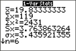 FIGURE 13 TI-83/84 output.
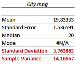 FIGURE 14 Excel output.
 FIGURE 15 Minitab output.
 FIGURE 16 JMP output.
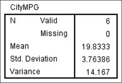 FIGURE 17 SPSS output.
Next, we turn to methods for applying the standard deviation.
4 The empirical rule
If the data distribution is bell-shaped, we may apply the Empirical Rule to find the approximate percentage of data that lies within standard deviations of the mean, for .
The empirical rule
If the data distribution is bell-shaped:
- About 68% of the data values will fall within 1 standard deviation of the mean.
- For a population, about 68% of the data will lie between and .
- For a sample, about 68% of the data will lie between and .
- About 95% of the data values will fall within 2 standard deviations of the mean.
- For a population, about 95% of the data will lie between and .
- For a sample, about 95% of the data will lie between and .
- About 99.7% of the data values will fall within 3 standard deviations of the mean.
- For a population, about 99.7% of the data will lie between and .
- For a sample, about 99.7% of the data will lie between and .
Figure 18 illustrates these approximate percentages.
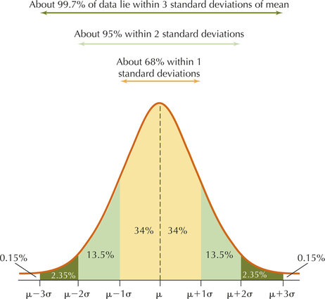
 Remember: The Empirical Rule may be applied only if the data distribution is bell-shaped.
EXAMPLE 15 Using the Empirical rule to find percentages
The College Board reports that the population mean Math SAT score for 2014 is , with a population standard deviation of . Assume the distribution of Math SAT scores is bell-shaped.
- Find the percentage of Math SAT scores between 396 and 632.
- Compute the percentage of Math SAT scores that are above 750.
Solution
- We see that a Math SAT score of 396 represents 1 standard deviation below the mean, becausePage 137
Remember: The English word “about” is not optional; it is required. The Empirical Rule is an approximation of normal distribution probabilities that we will examine more closely in Chapter 6.
Similarly, a Math SAT score of 632 represents 1 standard deviation above the mean, because
Thus, “Math SAT scores between 396 and 632” represents between and , that is, within 1 standard deviation of the mean. The data distribution is bell-shaped, so we may use the Empirical Rule. Therefore, about 68% of the Math SAT scores lie between 396 and 632, as shown in Figure 19.
We note that a Math SAT score of 750 represents 2 standard deviations above the mean, because
We know from the Empirical Rule that about 95% of the Math SAT scores lie within 2 standard deviations of the mean, so that about 95% of the Math SAT scores lie between 278 and 750. The left-over area of about 5% in the two tails in Figure 19 is the percentage of Math SAT scores above 750 or below 278. Because the bell-shaped curve is symmetric, the two tail areas are equal in area, which means that about 2.5% of the Math SAT scores lie above 750 (Figure 19).
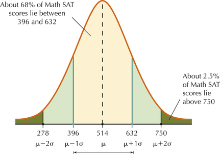 FIGURE 19 Example of Empirical Rule applied to Math SAT scores.
NOW YOU CAN DO
Exercises 23–30.
YOUR TURN#8
Suppose vehicle speeds on the local interstate highway are bell-shaped, with a mean of mph and a standard deviation of mph.
- Find the percentage of vehicle speeds between 65 mph and 75 mph.
- Compute the percentage of vehicles that are obeying the speed limit of at most 65 mph.
(The solutions are shown in Appendix A.)
5 Chebyshev's Rule
P. L. Chebyshev (1821-1894, Russia) derived a result, called Chebyshev's rule, that can be applied to any continuous data set.
Chebyshev's rule
The proportion of values from a data set that will fall within standard deviations of the mean will be at least
where . Chebyshev's Rule may be applied to either samples or populations. For example:
- When , at least 3/4 (or 75%) of the data values will fall within 2 standard deviations of the mean.
- When , at least 8/9 (or 88.89%) of the data values will fall within 3 standard deviations of the mean.

Because of the phrase “at least,” we say that Chebyshev's Rule provides minimum percentages, instead of the approximate percentages provided by the Empirical Rule. The actual percentage may be much greater than the minimum percentage provided by Chebyshev's Rule.
EXAMPLE 16 Using Chebyshev's Rule to find minimum percentages
The College Board reports that the population mean SAT Writing exam score for 2014 is , with a population standard deviation of . However, assume we do not know the data distribution. Find the minimum percentage of exam scores that is
- between 260 and 716.
- between 317 and 659.
- between 374 and 602.
Solution
The data distribution is unknown, so we cannot apply the Empirical Rule.
- Because 260 lies 2 standard deviations below the mean
and 716 lies 2 standard deviations above the mean
this question is really asking what is the minimum percentage within standard deviations of the mean. From Chebyshev's Rule, the minimum percentage is
Thus, at least 75% of the SAT Writing exam scores will lie between 260 and 716.
- The exam scores 317 and 659 lie standard deviations below and above the mean, respectively. Therefore, at least
of the SAT Writing exam scores will lie between 317 and 659.
Page 139 - The scores 374 and 602 lie standard deviation below and above the mean, respectively. Unfortunately, Chebyshev's Rule is restricted to situations where . Thus, we cannot answer this question.
NOW YOU CAN DO
Exercises 31–38.
Developing Your Statistical Sense
Strengths and Weaknesses of the Empirical Rule and Chebyshev's Rule
Example 16 shows that the lack of knowledge of a bell-shaped distribution can have a cost.
- For part (a), using the Empirical Rule with would have given us an answer of “about 95%,” which is more precise than “at least 75%.” However, this extra precision comes only if we know the distribution is bell-shaped.
- For part (b), however, the Empirical Rule does not apply to any values other than 1, 2, or 3, so would have been no help here.
- Finally, had we been able to apply the Empirical Rule in part (c), then we could have gotten an answer of “about 68%” for .
YOUR TURN#9
Suppose systolic blood pressure in a population of senior citizens has a mean of and a standard deviation of . Find the minimum percentage of systolic blood pressure readings between 110 and 150.
(The solution is shown in Appendix A.)
If a given data set is bell-shaped, either the Empirical Rule or Chebyshev's Rule may be applied to it.
 Can the Financial experts Beat the Darts?
Recall from the Case Study at the beginning of this chapter, the Wall Street Journal competition between stocks chosen randomly by Journal staff members throwing darts and stocks chosen by a team of four fnancial experts. Note from Figure 20 that the DJIA exhibits less variability than the other two portfolios. This smaller variability is due to the fact that the DJIA is made up of 30 component stocks, whereas each portfolio is made up of only four stocks. Smaller sample sizes can be associated with increased variability, because an unusual result in one value has a relatively strong effect on the mean when it is not offset by a large sample.
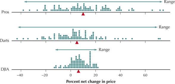
Which of the portfolios, pros or darts, shows greater variability? It is difficult to determine which has the greater standard deviation, just by examining Figure 20. We therefore turn to the Minitab descriptive statistics in Figure 21. The range for the darts, 115.90, is greater than the range for the pros, 112.80. But the standard deviation for the darts (19.39) is less than that of the pros (22.25).
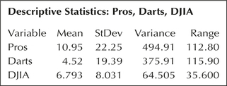
Measures of spread may disagree about which data set has more variability. However, the range takes into account only the two most extreme data values; therefore, the standard deviation is the preferred measure of spread because it uses all the data values. Our conclusion, therefore, is that the returns for the professionals exhibit a greater variability.
Why did the pros have more variability than the darts? After all, in finance, high variability is not necessarily advantageous because it is associated with greater risk. The professionals evidently chose higher-risk stocks with greater potential for high returns—but also greater potential for losing money.