3 Describing Data Numerically

3.3 Working with Grouped Data

OBJECTIVES By the end of this section, I will be able to …

Calculate the weighted mean.
Estimate the mean for grouped data.
Estimate the variance and standard deviation for grouped data.

1 The weighted Mean

Note: Before tackling this section, you may wish to review Section 2.2, “Graphs and Tables for Quantitative Data” (page 60).

Sometimes, not all the data values in a data set are of equal importance. Certain data values may be assigned greater importance or weight than others when calculating the mean. For example, have you ever figured out what your final grade for a course was based on the percentages listed in the syllabus? What you actually found was the weighted mean of your grades.

Page 149

Note: The weights, $w$ , do not have to be percentages, nor do they have to add up to 1.

In the special case when all the weights equal 1, the weighted mean equals the sample mean $\bar{x}$ from Section 3.1.

Weighted Mean

To find the weighted mean:

Multiply each weight, $w$ , by its corresponding data value, $x$ .
Add up the products to get $\sum (w \cdot x)$ .
Divide the result by the sum of the weights, $\sum w$ .
$\bar{x} = \frac{\sum (w . x)}{\sum w}$

EXAMPLE 17 weighted mean of course grades

The syllabus for the Introduction to Management course at a local college specifies that the midterm exam is worth 30%, the term paper is worth 20%, and the final exam is worth 50% of your course grade. Now, say you did not get serious about the course until after Halloween, so that you got a 40 on the midterm. You then began working harder, and got a 70 on the term paper. Finally, you remembered that you had to pay for the course again if you did not pass and had to retake it, so you worked really hard for the last month of the course and got a 90 on the final exam. Calculate your course average, that is, the weighted mean of your grades.

Solution

The data values are 40, 70, and 90. The weights are 0.30, 0.20, and 0.50. Your course weighted mean is then calculated as follows:

$\bar{x} = \frac{\sum (w . x)}{\sum w} = \frac{(0.30) (40) + (0.20) (70) + (0.50) (90)}{0.30 + 0.20 + 0.50} = \frac{71}{1.0} = 71$

Because the final exam had the most weight, you were able to raise your course weighted mean to 71, and you passed the course.

NOW YOU CAN DO

Exercises 4–8.

YOUR TURN#10

The author's syllabus for his Business Statistics I course during Summer 2014 stated that the quiz average was worth 50% of the course grade, with the midterm worth 20% and the final exam worth 30%. One of the students had a 90 quiz average, a 70 midterm grade, and an 85 final exam grade. Calculate the student's course grade.

(The solution is shown in Appendix A.)

2 Estimating the Mean for grouped Data

Thus far in Chapter 3, we have computed measures of center and spread from a raw data set. However, data are often reported using grouped frequency distributions. Without the original data, we cannot calculate the exact values of the measures of center and spread. The remainder of this section examines methods for approximating the mean, variance, and standard deviation of grouped data— that is, population data summarized using frequency distributions.

For each class in the frequency distribution, we estimate the class mean using the class midpoint. The class midpoint, denoted $x$ , is defned as the mean of two adjoining lower class limits.

The product of the class frequency, $f$ , and class midpoint, $x$ , is used as an estimate of the sum of the data values within that class. Summing these products across all classes and dividing by the size of the data set thus provides us with an estimated mean for data grouped into a frequency distribution.

Page 150

Note: Even though we are working with population data, we will notate these values using $\bar{x}$ and $s$ because we are estimating the values of the mean and standard deviation.

Estimated Mean for Data grouped into a Frequency Distribution

Given a population frequency distribution, the estimated mean for the variable is given by

$\bar{x} = \frac{\sum (f . x)}{\sum f}$

where $x$ and $f$ represent the class midpoints and class frequencies, respectively.

EXAMPLE 18 Calculating the estimated mean for grouped data

The first two columns of Table 17 contain the frequency distribution of the number of Americans younger than 85 years old who were living in the United States in 2013, by age group, as reported by the U.S. Census Bureau.

Find the class midpoints.
Calculate the product of each class frequency with its midpoint.
Find the sum of the frequencies, $\sum f$ , and the sum of the products, $\sum (f \cdot x)$ .
Divide $\sum (f \cdot x)$ by $\sum f$ to find the estimated mean age of all Americans under the age of 85.

Solution

The midpoint for the first class (ages 0–20) is the mean of the lower class limits for this class (0) and the adjoining class (20). That is, the midpoint is $(0 + 20) / 2 = 10$ . Similarly, the midpoint for the second class (ages 20–40) is $(20 + 40) / 2 = 30$ . The remainder of the class midpoints are calculated in the same way and are shown in Table 17.
We multiply the frequency for the first age group by its midpoint to get $83.3 \cdot 10 = 833$ . We do the same for the other age groups, as shown in Table 17.
We add up all the frequencies to get $\sum f = 303.3$ . Also, we add up all the products from (b) to obtain $\sum (f \cdot x) = 11, 338$ .
Finally, obtain the estimated mean, as follows:
$\bar{x} = \frac{\sum (f . x)}{\sum f} = \frac{11, 338}{303.3} = 37.4$

The estimated mean age of all Americans under 85 is 37.4 years.

Table 3.63: Table 17 Frequency distribution of Americans, by age group, in millions

Class: age	Frequency $f$	Midpoint $x$	Product $f \cdot x$
$0 \leq age < 20$	83.3	10	$83.3 \cdot 10 = 833$
$20 \leq age < 40$	82.8	30	$82.3 \cdot 30 = 2,484$
$40 \leq age < 60$	85.6	50	$85.6 \cdot 50 = 4,280$
$60 \leq age < 85$	51.6	72.5	$51.6 \cdot 72.5 = 3,741$
Total	$\sum f = 303.3$		$\sum (f \cdot x) = 11, 338$

NOW YOU CAN DO

Exercises 9–14.

Page 151

3 Estimating the Variance and Standard Deviation for Grouped Data

We also use class midpoints and class frequencies to calculate the estimated variance for data grouped into a frequency distribution and the estimated standard deviation for data grouped into a frequency distribution.

Estimated Variance and Standard Deviation for Population Data Grouped into a Frequency Distribution

The estimated variance for data grouped into a frequency distribution is given by

$s^{2} = \frac{{\sum (x - \bar{x})}^{2} . f}{\sum f}$

and the estimated standard deviation is given by

$s = \sqrt{s_{\cdot}^{2}} = \sqrt{\frac{{\sum (x - \bar{x})}^{2} . f}{\sum f}}$

where $x$ represents the class midpoints, $f$ represents the class frequencies, and $\bar{x}$ is the estimated mean.

You should carry as many decimal places as you can for the value of $\bar{x}$ when calculating $s^{2}$ , and for $s^{2}$ when calculating $s$ .

EXAMPLE 19 Calculating the estimated variance and standard deviation for grouped data

Calculate the estimated variance and standard deviation of the ages of Americans under age 85 from Table 17.

Solution

Table 18 contains the calculations required for finding ${\sum (x - \bar{x})}^{2} \cdot f = 144, 234$ . The variance is therefore estimated as

$s^{2} = \frac{{\sum (x - \bar{x})}^{2} . f}{\sum f} = \frac{144, 234}{303.3} \approx 475.5487$

and the standard deviation is estimated as

$s = \sqrt{s^{2}} = \sqrt{475.5487} \approx 21.8$

Table 3.64: Table 18 Calculating

${\sum (x - \bar{x})}^{2} \cdot f$

Class: age	Midpoint $x$	Frequency $f$	$\bar{x}$	$x - \bar{x}$	${(x - \bar{x})}^{2} \cdot f$
$0 \leq age < 20$	10.0	83.3	37.4	−27.4	62,538.31
$20 \leq age < 40$	30.0	82.8	37.4	−7.4	4,534.13
$40 \leq age < 60$	50.0	85.6	37.4	12.6	13,589.86
$60 \leq age < 85$	72.5	51.6	37.4	35.1	63,571.72
				$\sum {(x - \bar{x})}^{2} \cdot f = 144, 234$

In other words, the age of Americans under 85 typically differs from the mean age of 37.4 years by about 21.8 years.

NOW YOU CAN DO

Exercises 15–20.

Page 152

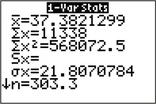
EXAMPLE 20 Using technology to find the estimated mean, variance, and standard deviation for grouped data

Use the TI-83/84 calculator to find the estimated mean, variance, and standard deviation for the frequency distribution in Table 17.

Solution

Following the instructions in the Step-by-Step Technology Guide, we get the estimated mean, $\bar{x} = 37.3821299$ (which we round to 37.4), the estimated standard deviation, $s$ (shown in the output as $σ_{x}$ ) $= 21.8070784$ , and the estimated variance as ${(21.8070784)}^{2} = 475.5487$ .

usa-ages