6.6Normal Approximation to the Binomial Probability Distribution
 This page includes Statistical Videos
OBJECTIVES By the end of this section, I will be able to …
- Use the normal distribution to approximate probabilities of the binomial distribution.
1Using the Normal Distribution to Approximate Probabilities of the Binomial Distribution
Recall from Section 6.2 that a binomial experiment satisfies the following four requirements: (1) Each trial must have two possible outcomes. (2) There is a fixed number of trials, n. (3) The experimental outcomes are independent. (4) The probability of observing a success is the same from trial to trial.
For certain values of n and p, it may be inconvenient to calculate probabilities for the binomial distribution. For example, if we are flipping a fair coin 100 times, so that n=100 and p=0.5, it may be tedious to calculate P(X≥57), which, in the absence of technology, would involve 44 applications of the binomial probability formula. Fortunately, if the requirements are met, we may use the normal distribution to approximate such probabilities.
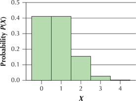
The binomial random variable X represents the number of successes in n trials and thus depends on the sample size n and the probability of success p. For a given probability of success p, if the sample size n gets large enough, the binomial distribution begins to resemble the normal distribution. Figure 71 shows the binomial probability distribution for Example 16 (page 330), where 20% (p=0.2) of Americans are sleep-deprived and we sampled n=4 Americans. The distribution of X = the number of Americans who are sleep-deprived in Figure 71 is clearly not normal.
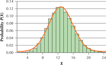
If we increase the sample size to n=64 (Figure 72), the binomial distribution of X for n=64 and p=0.2, which is discrete, looks like it can be nicely approximated by the normal distribution, which is continuous.
We generalize this behavior as follows.
The Normal Approximation to the Binomial Probability Distribution
For the binomial random variable X with probability of success p and number of trials n: if n⋅p≥5 and n⋅q≥5, the binomial distribution may be approximated by a normal distribution with mean μX=n⋅p and standard deviation σX=√n⋅p⋅q.
These values for μx and σx are the same as the values for μ and σ for a binomial random variable that we learned about on page 334.
EXAMPLE 44The normal approximation to the binomial distribution

The Centers for Disease Control and Prevention reported that 20% of preschool chil dren lack required immunizations, thereby putting themselves and their classmates at risk. For a group of n=64 children with p=0.2, the binomial probability distribution is shown in Figure 72.
- Verify that this distribution can be approximated by a normal distribution.
- Find the mean and standard deviation of this normal distribution.
Solution
- The normal approximation is valid if n⋅p≥5 and n⋅q≥5. Substituting n=64 and p=0.2, we get n⋅p=(64)(0.2)=12.8≥5andn⋅q=(64)(0.8)=51.2≥5
Thus, the normal approximation is valid.
The mean and standard deviation of the normal distribution are
μx=n⋅p=(64)(0.2)=12.8σx=√n⋅p⋅q=√(64)(0.2)(0.8)=3.2
NOW YOU CAN DO
Exercises 3–8.
Figure 73 reproduces Figure 72, with the rectangle for X=12 highlighted. The height of the rectangle represents the binomial probability that exactly 12 of the 64 children lack the required immunizations, that is, P(X=12). The width of the rectangle equals 12.5−11.5=1 , so it follows that the area of the rectangle also represents the binomial probability that X=12. Now, the area under the normal curve between 11.5 and 12.5 is approximately equal to this rectangle, which is P(X>X12) for the binomial random variable X, with n=64 and p=0.2. That is,
P(Xbinomial=12)≈P(11.5≤Ynormal≤12.5)
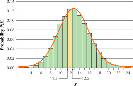
where Ynormal is the normal random variable from Example 44(b), with mean μx=12.8 and standard deviation σx=3.2.
The 0.5 that we add and subtract from 12 when approximating the binomial distribution with the normal distribution is called the continuity correction, because it is an adjustment for approximating a discrete probability with a continuous one. When using the normal approximation to the binomial, the analyst must determine which binomial rectangles are included and apply the continuity correction accordingly. This is shown in Table 9, which provides a listing of several types of binomial probabilities and their normal probability approximations.
| Exact binomial probability | Approximate normal probability |
|---|---|
| P(Xbinomial=a) | P(a−0.5≤Ynormal≤a+0.5) |
| P(Xbinomial≤a) | P(Ynormal≤a+0.5) |
| P(Xbinomial≥a) | P(Ynormal≥a−0.5) |
| P(Xbinomial<a) | P(Ynormal<a−0.5) |
| P(Xbinomial>a) | P(Ynormal>a−0.5) |
| P(a≤Xbinomial≤b) | P(a−0.5≤Ynormal≤b+0.5) |
| P(a<Xbinomial<b) | P(a+0.5<Ynormal<b−0.5) |
EXAMPLE 45Performing the normal approximation to the binomial probability distribution
For a group of n=64 preschool children with the probability of lack of immunization p=0.2, perform the following approximations:
- Approximate the probability that there are, at most, 12 children without immunizations.
- Approximate the probability that there are more than 12 children without immunizations.
Solution
Once again, we have a binomial experiment with n=64 and p=0.2.
“At most” 12 children means 12 or fewer children. That is, X=12 and X=11 and X=10, and so on; that is, P(Ybinomial≤12). In this case, we see that X=12 is included in the probability we seek, as shown in Figure 74. From Table 9, we see that P(Xbinomial≤12) is of the form P(Xbinomial≤a). Thus, our continuity correction takes the form P(Ynormal≤a+0.5), where we add 0.5 to 12, so that
P(Xbinomial≤12)≈P(Ynormal≤12.5)
Recall that μx=12.8 and σx=3.2. We use the TI-83/84, as shown in Figures 75 and 76, and find that the probability that, at most, 12 children lack immunizations is 0.462653813≈0.4627.
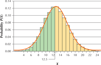 FIGURE 74 Approximates a binomial probability with a normal probability.
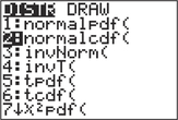 FIGURE 75 TI-83/84.
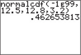 FIGURE 76 TI-83/84 results.
“More than” 12 children means X=13 and X=14, and so on. In other words, X=12 is not included. That is, we want P(Xbinomial>12). From Table 9, we see that P(Xbinomial>12) is of the form P(Xbinomial>a). Thus, our continuity correction takes the form P(Ynormal>a+0.5), where we add 0.5 to 12, so that
P(Xbinomial>12)≈P(Ynormal>12.5)
The desired area is the complement of the green area in Figure 74, so we can find the answer like this:
P(Xbinomial>12)≈P(Ynormal>12.5)=1−P(Ynormal≤12.5)=1−0.4627=0.5373
The probability that more than 12 preschool children will not have the required immunizations is 0.5373.
![]() The Normal Approximation to the Binomial Distributions applet allows you to choose your own values of n and p and see how changes in these values affect the normal approximation to the binomial distribution.
The Normal Approximation to the Binomial Distributions applet allows you to choose your own values of n and p and see how changes in these values affect the normal approximation to the binomial distribution.
NOW YOU CAN DO
Exercises 9–24.
YOUR TURN#23
For the scenario in Example 45, approximate the probability that there are less than 12 children without immunizations.
(The solution is shown in Appendix A.)