1. Explain what constitutes a binomial experiment.
2. Compute probabilities using the binomial probability formula, binomial tables, and technology.
3. Calculate the mean, variance, and standard deviation of the binomial random variable and find the mode of the distribution.

1. Each trial of the experiment has only two possible mutually exclusive outcomes (or is defined in such a way that the number of outcomes is reduced to two). One outcome is denoted a success and the other a failure.
2. A fixed number of trials exists, which is known in advance of the experiment.
3. The experimental outcomes are independent of each other.
4. The probability of observing a success remains the same from trial to trial.

Many experiments having more than two outcomes can often be defined so that only two outcomes are possible. For example, the answer to a multiple-choice question that has five answer choices may be recorded as either correct or incorrect.

1. A fisherman is going fishing and will continue to fish until he catches a rainbow trout.
2. We flip a fair coin three times and observe the number of heads.
3. A market researcher at a shopping mall is asking consumers whether they use Fib detergent. She asks a sample of four men, one of whom is clearly the employer of the other three.
4. The National Burglar and Fire Alarm Association reports that 34% of burglars get in through the front door. A random sample of 36 burglaries is taken, and the number of entries through the front door is noted.

1. This is not a binomial experiment because you don't know how many fish he will catch before the rainbow trout shows up, so a fixed number of trials isn't known in advance.

2. This is a binomial experiment because it fulfills the requirements:

   1. Only two possible outcomes are possible on each trial, with heads defined as success and tails as failure.
   2. We know in advance that we are tossing the coin three times.
   3. The coin doesn't remember its result from toss to toss, and so the trials are independent.
   4. The coin is fair on each toss, and so the probability of observing heads is the same on each toss.

   The binomial random variable $X$ is the number of heads observed on the three trials; because the coin is fair, the probability of success is 0.5 and the probability of failure is 0.5. The possible values for $X$ are 0, 1, 2, or 3.

3. This is not a binomial experiment because the responses are not independent. The response given by the employer is likely to affect the employees' responses.

4. This is a binomial experiment because it fulfills the requirements:

   1. Only two possible outcomes are possible on each trial: entering through the front door or not entering through the front door.
   2. We know in advance that the size of the random sample is 36 burglaries.
   3. The sample is random, so the trials are independent.
   4. The sample is quite small compared to the size of the population, so the probability of entering through the front door remains the same from burglary to burglary.

Note: In Section 5.4, we used ${}_n{C}_r$ to indicate the number of combinations. Now that we have learned about random variables, which can be denoted $X$, we use ${}_n{C}_X$ to represent the number of combinations.

Note: You may find the following special combinations useful. For any integer $n$:

$\begin{array}{cc}{}_n{C}_n=1& {}_n{C}_0=1\\ {}_n{C}_1=n& {}_n{C}_{n-1}=n\end{array}$

${}_n{C}_X=\frac{n!}{X!(n-X)!}$

$X=\text{the number of "LTRers"}$

1. Construct a tree diagram for this experiment.
2. Suppose that we are interested in finding the probability that exactly two of the three online daters would be LTRers, $P(X=2)$. In the tree diagram, highlight in blue the outcomes where exactly two of the three online daters are LTRers. Find the probability for each outcome, and use these to find $P(X=2)$.
3. Suppose that we are interested in finding $P(X=1)$. In the tree diagram, highlight in red the outcomes where exactly one of the three online daters is an LTRer. Find the probability for each outcome, and use these to find $P(X=1)$.

1. Figure 7 shows the tree diagram for this experiment.

2. As we can see from Figure 7, there are $\left({{\displaystyle }}_n{C}_x\right)=\left({{\displaystyle }}_3{C}_2\right)=3$ different ways that exactly two of the three online daters could be LTRers (highlighted in blue).

   FIGURE 7 Tree diagram and binomial probabilities.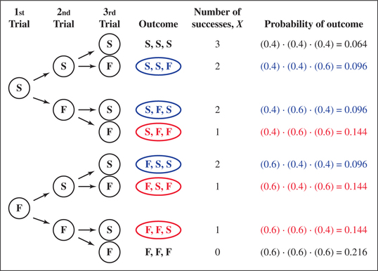

   
   Page 330

   For each of these three outcomes, the probability that $X=2$ is ${\left(0.4\right)}^2\left(0.6\right)=0.096$.

   • The outcome $S,S,F$ (second row in Figure 7) has probability $\left(p\right)\left(p\right)\left(q\right)=\left(0.4\right)\left(0.4\right)\left(0.6\right)=0.096$.
   • The outcome $S,F,S$ has probability $\left(p\right)\left(q\right)\left(p\right)=\left(0.4\right)\left(0.6\right)\left(0.4\right)=0.096$.
   • The outcome $F,S,S$ has probability $\left(q\right)\left(p\right)\left(p\right)=\left(0.6\right)\left(0.4\right)\left(0.4\right)=0.096$.

   Note that each of these products equals ${\left(p\right)}^2.q$, with $p$ having exponent $X=2$, and ($q$) having exponent $n-X=3-2=1$. Thus,

   $\begin{array}{l}P(X=2)={(}_3{C}_2\left)\right(0.4{)}^2\left(0.6\right)\\ =3\left(0.096\right)=0.288\end{array}$

3. Similarly, suppose that we are interested in whether exactly one $(X=1)$ of the three online daters is an LTRer. Then, Figure 7 shows us, highlighted in red, that there are ${(}_n{C}_X)={(}_3{C}_1)=3$ different ways this could happen. Each of these outcomes has probability $\left(p\right)\cdot {\left(q\right)}^2=\left(0.4\right){\left(0.6\right)}^2=0.144$, where $p$ has exponent $X=1$, and $q$ has exponent $n-X=3-1=2$. Thus,

   $\begin{array}{l}P(X=1)={(}_3{C}_1\left)\right(0.4){\left(0.6\right)}^2\\ =3\left(0.144\right)=0.432\end{array}$

$P\left(X\right)={(}_n{C}_X)p^X{\left(q\right)}^{n-X}$

$P\left(X\right)={(}_n{C}_X\left)\right[P{(\text{success)}}^{\text{number of successes}}\cdot P{(\text{failure)}}^{\text{number of failures}}].$

• Step 1 Find the number of trials $n$, and the probability of success on a given trial $p$.
• Step 2 Find the number of successes $X$ about which the question is asking.
• Step 3 Using the values from Steps 1 and 2, find the required probabilities using either the binomial probability formula, the binomial tables (which we learn below), or technology.

1. None
2. At least one
3. Between one and three, inclusive
4. Five

• Step 1 We have a random sample of four Americans, so the number of trials is $n=4$. “Success” is denoted as a particular American being sleep-deprived. The report states that 20% of Americans are sleep-deprived, so $p=0.2$ and $q=1-0.2=0.8$.
• Step 2 For (a), $X=0$. For (b), $X\ge 1$; that is, $X=1,2,3,\text{or}4$. For (c), $1\le X\le 3$; that is, $X\ge 1$; that is, $X=1,2,3$. For (d), $X=5$.
• Step 3 We apply Step 3 for each of (a)–(d) as follows:

1. Step 3 To find the probability that none ($X=0$) of the Americans are sleep-deprived, we use the binomial probability formula:

   $P(X=0)={(}_4{C}_0){\left(0.2\right)}^0{\left(0.8\right)}^{4-0}=(1\left)\right(1\left)\right(0.4096)=0.4096$

   Therefore, the probability that none of the Americans in the sample are sleep-deprived is 0.4096.

2. Step 3 Note that “at least one” includes all possible values of $X$ except $X=0$. In other words, the two events ($X=0$) and ($X\ge 1$) are complements of each other. Therefore, from the formula for the probability for complements in Section 5.2 (page 260), we have

   $P(x\ge 1)=1-P(X=0)=1-0.4096=0.5904$

   The probability that at least one of the Americans is sleep-deprived is 0.5904.

3. Step 3 We need to find the probability that either $X=1$ or $X=2$ or $X=3$ of the Americans are sleep-deprived. Because these three values of $X$ are mutually exclusive, we find the required probability by using the Addition Rule for Mutually Exclusive Events.

   $\begin{array}{l}P(1\le X\le 3)=P(X=1\text{or}X=2\text{or }X=3)\\ =P(X=1)+P(X=2)+P(X=3)\end{array}$

   So we calculate the following:

   $\begin{array}{l}P(X=1)={(}_4{C}_1\left)\right(0.2{)}^1(0.8{)}^{4-1}=(4\left)\right(0.2\left)\right(0.512)=0.4096\\ P(X=2)={(}_4{C}_2\left)\right(0.2{)}^2(0.8{)}^{4-2}=(6\left)\right(0.04\left)\right(0.64)=0.1536\\ P(X=3)={(}_4{C}_3\left)\right(0.2{)}^2(0.8{)}^{4-3}=(4\left)\right(0.08\left)\right(0.8)=0.0256\end{array}$

   Thus, $P(1\le X\le 3)=0.4096+0.1536+0.0256=0.5888$. The probability is 0.5888 that between one and three, inclusive, of the Americans in the sample of four are sleep-deprived.

4. Step 3 In a binomial experiment, the number of successes $X$ can never exceed the number of trials $n$. In other words, $X\le n$, always. So, if our sample has only $n=4$ Americans, then $P(X=5)=0$. It is not possible for there to be five Americans who are sleep-deprived.

YOUR TURN#8

1. 0
2. 1
3. At most 1

1. No Americans are sleep-deprived.
2. At least one American is sleep-deprived.

1. From Example 16, we have a binomial distribution with $n=4$ and $p=0.2$. We next find $n$ and $p$ in the binomial table. In Figure 8:
   • Look under the $n$ column until you find $n=4$. That is the portion of the table you will use.
   • Then go across the top of the table until you get to $p=0.20$.
   • For part (a), $X=0$, so go down the $X$ column until you see 0 under the $X$ column on the left (and in the subgroup with $n=4$).
   • The number in the $p$ column is 0.4096 (see Figure 8), which is the same answer we calculated in Example 16(a).
     FIGURE 8 Excerpt from the binomial tables.

     
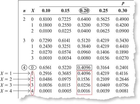
2. In this case, “at least 1” means 1 or 2 or 3 or 4. So, by the Addition Rule for Mutually Exclusive Events, find the probabilities for $X=1$, $X=2$, $X=3$, and $X=4$, and add them up. Using the same column with column head 0.20 in the table as in part (a), we add up the four probabilities.
   

   $\begin{array}{l}P(X\ge 1)=P(X=1)+P(X=2)+P(X=3)+P(X=4)\\ =0.4096+0.1536+0.0256+0.0016=0.5904\end{array}$

1. $P(X=4)$, the probability that all four Americans are sleep-deprived.
2. $P(X\le 2)$, the (cumulative) probability that, at most, two Americans are sleep-deprived.

1. Figure 9 shows that we use the TI-83/84 function binompdf with $n=4$, $p=0.2$, and $X=4$. Figure 10 shows the result: $P(X=4)=0.0016$. Figure 11 shows the same input and final answer using CrunchIt!.
   

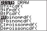   FIGURE 9 TI-83/84 menu.
   

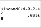   FIGURE 10 TI-83/84 result.
   

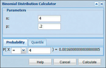   FIGURE 11 CrunchIt!
2. With the TI-83/84, we use the function binomcdf with $n=4$, $p=0.2$, and $X=2$. Figure 12 shows the result: $P(X\le 2)=0.9728$. Figure 13 shows the input and final answer using CrunchIt!.
   

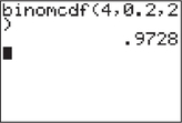   FIGURE 12 TI-83/84 result.
   

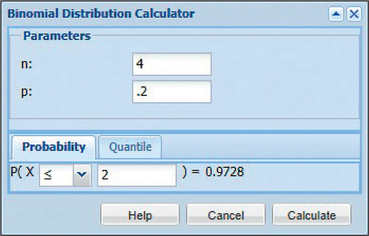   FIGURE 13 CrunchIt!

YOUR TURN#9

1. $P(X\le 5)$
2. $P(X<6)$
3. $P(0\le X\le 5)$
4. $P(0<X<5)$

• Mean (or expected value): $\mu =\eta \cdot p$
• Variance: ${\sigma }^2=\eta \cdot p\cdot q$
• Standard deviation: $\sigma =\sqrt{\eta \cdot p\cdot q}$

These formulas work only for a binomial random variable.

YOUR TURN#10

1. Find the mean $\mu$.
2. Calculate the variance ${\sigma }^2$ and standard deviation $\sigma$.
3. In a sample of 50, would it be unusual to observe $X=36$? (The solutions are shown in Appendix A.)

What Do $\mu$ and $\sigma$ Mean?

1. Calculate the mean number $\mu$ of American adults who use their cell phones to access the Internet.
2. Use the binomial table to construct a probability distribution graph of the random variable X = the number of Americans who use their cell phones to access the Internet.
3. Use the binomial table or the probability distribution graph to find the most likely number of American adults who use their cell phones to access the Internet. Note that this represents the mode of the distribution.

1. $\mu =n\cdot p=\left(3\right)\left(0.6\right)=1.8$
2. Figure 14 is an excerpt from the binomial table, highlighting the probabilities for $X=0,1,2\text{, and}3$, for $n=3$ and $p=0.6$. We use these probabilities to construct the probability distribution graph shown in Figure 15.
   Page 336
   

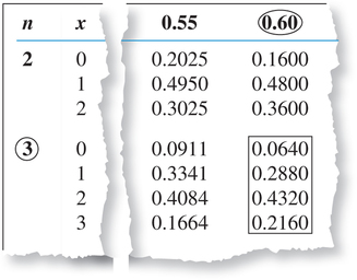   FIGURE 14 Probabilities for $X=0,1,2,3$.
   

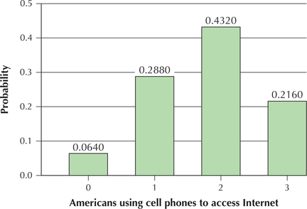   FIGURE 15 Probability distribution graph of $X$.
3. The most likely number of Americans using their cell phones to access the Internet is associated with the largest probability in the boxed section of Figure 14, 0.4320, which is $P(X=2)$. Note from Figure 15 that $X=2$ has the tallest bar of probability. Thus, $X=2$ is the most likely number of American adults using their cell phones to access the Internet. We say that $X=2$ is the mode of the distribution of $X$.