Section 6.2Exercises
CLARIFYING THE CONCEPTS
Question 6.99
1. State the four requirements for a binomial experiment. (p. 327)
6.2.1
(i) Each trial of the experiment has only two possible mutually exclusive outcomes (or is defined in such a way that the number of outcomes is reduced to two). One outcome is denoted a success and the other a failure. (ii) There is a fixed number of trials, known in advance of the experiment. (iii) The experimental outcomes are independent of each other. (iv) The probability of observing a success remains the same from trial to trial.
Question 6.100
2. What is meant by a “success” in a binomial experiment? Is a success always a good thing? (p. 328)
Question 6.101
3. In a binomial experiment, explain why it is not possible for X to exceed n. (p. 327)
6.2.3
If you perform an experiment n times, you can't have more than n successes. For example, if you flip a coin 10 times you can't get 11 heads.
Question 6.102
4. Restate the binomial probability distribution formula using the following terms: nCx, the probability of success, the number of successes, the probability of failure, and the number of failures. (p. 330)
PRACTICING THE TECHNIQUES
 CHECK IT OUT!
| To do | Check out | Topic |
|---|---|---|
| Exercises 5–14 |
Example 14 | Recognizing binomial experiments |
| Exercises 15–28 |
Example 16 | Applying the binomial probability distribution formula |
| Exercises 29–48 |
Examples 17 and 18 | Finding binomial probabilities using table or technology |
| Exercises 49–52 |
Example 19 | Binomial mean, variance, and standard deviation |
| Exercises 53–56 |
Example 20 | The binomial mode: the most likely outcome of a binomial experiment |
For Exercises 5–14, determine whether the experiment is binomial or not. If the experiment is binomial, identify the random variable X, the number of trials n, the probability of success p and the probability of failure q. If the experiment is not binomial, explain why not.
Question 6.103
5. Ask 10 of your friends to come to your party (remember the independence assumption on page 327).
6.2.5
Not binomial; the events “Person A comes to party” and “Person B comes to party” may not be independent.
Question 6.104
6. Toss a fair die three times, and note the total number of spots.
Question 6.105
7. Answer a random sample of eight multiple-choice questions either correctly or incorrectly by random guessing. There are four choices, (a)-(d), for each question.
6.2.7
Binomial, X=number of correct answers, n=8,p=1/4=0.25,1−p=3/4=0.75
Question 6.106
8. Toss a fair die three times, and note the number of 6s.
Question 6.107
9. Select a student at random in the class until you come across a left-handed student.
6.2.9
Not binomial; not a fixed number of trials
Question 6.108
10. Four cards are selected at random with replacement from a deck of cards, and the number of queens is observed.
Question 6.109
11. Four cards are selected at random without replacement from a deck of cards, and the number of queens is observed.
6.2.11
Not binomial, trials are not independent, sample is more than 1% of the population.
Question 6.110
12. Four cards are selected at random with replacement from a deck of cards, and the total number of blackjack-style points (number cards = number of points; face cards = 10 points; aces = either 1 or 11) is calculated.
Question 6.111
13. Bob has paid to play two games at a carnival. The probability that he wins a particular game is 0.25.
6.2.13
Binomial; n=2, X=number of games won, p=0.25, 1−p=0.75
Question 6.112
14. Bob is playing a game at a carnival where he gets to play until he loses. The probability that he wins a particular game is 0.25.
For Exercises 15–28, calculate the probability of X successes for the binomial experiments with the following characteristics:
Question 6.113
15. n=5,p=0.25,X=1
6.2.15
0.3955
Question 6.114
16. n=5,p=0.25,X=0
Question 6.115
17. n=10,p=0.5,X=7
6.2.17
0.1172
Question 6.116
18. n=10,p=0.5,X=8
Question 6.117
19. n=12,p=0.9,X=10
6.2.19
0.2301
Question 6.118
20. n=12,p=0.9,X=11
Question 6.119
21. n=5,p=0.25,X≤1
6.2.21
0.6328
Question 6.120
22. n=5,p=0.25,X≥1
Question 6.121
23. n=10,p=0.5,X=7 or X=8
6.2.23
0.1611
Question 6.122
24. n=10,p=0.5,X=7 and X=8
Question 6.123
25. n=12,p=0.9,X≥10
6.2.25
0.8891
Question 6.124
26. n=12,p=0.9,X<10 (Hint: Use the result from Exercise 25.)
Question 6.125
27. n=12,p=0.9,9≤X≤12
6.2.27
0.9744
Question 6.126
28. n=12,p=0.9,8≤X≤12
According to the National Center for Education Statistics, business majors accounted for 25% of the proportion of all Master's degrees granted in 2012. For Exercises 29–34, the binomial experiment is to select three Master's degrees at random and to observe X = number of business majors. Calculate the indicated probabilities.
Question 6.127
29. Observe no business majors
6.2.29
0.421875
Question 6.128
30. Observe one business major
Question 6.129
31. Observe two business majors
6.2.31
0.140625
Question 6.130
32. Observe at most two business majors
Question 6.131
33. Observe at least one business major
6.2.33
0.578125
Question 6.132
34. Observe between zero and two business majors, inclusive
A study by the Centers for Disease Control and Prevention (Use of Medication Prescribed for Emotional or Behavioral Difficulties Among Children Aged 6-17 Years in the United States, 2011-2012, by LaHeana Howie et al., NCHS Data Brief Number 148, April 2014) showed that 7.5% of children ages 6-17 used prescribed medication during the past six months for emotional or behavioral difficulties. For Exercises 35–40, the binomial experiment is to select four children ages 6-17 at random, and to find the probability that X takes the following values, where X = the number of children using prescription medication for emotional or behavioral difficulties:
Question 6.133
35. X=3
6.2.35
0.0015609375
Question 6.134
36. X≥3
Question 6.135
37. X=0
6.2.37
0.7320941406
Question 6.136
38. X≤1
Question 6.137
39. 1≤X≤4
6.2.39
0.2679058594
Question 6.138
40. 1<X<4
According to the Current Population Survey, 10% of Americans ages 25-29 live alone. For Exercises 41–44, the binomial experiment is to take a random sample of five Americans ages 25-29 and observe X = the number living alone. Find the indicated probabilities.
Question 6.139
41. None are living alone.
6.2.41
0.59049
Question 6.140
42. At least one is living alone.
Question 6.141
43. At most two are living alone.
6.2.43
0.99144
Question 6.142
44. Six are living alone.
A 2014 study by the Harvard University Institute of Politics found that 40% of 18- to 29-year olds had a Twitter account. For Exercises 45–48, suppose we take a random sample of six 18- to 29-year-olds and find X = the number who have a Twitter account. Find the following probabilities:
Question 6.143
45. X=6
6.2.45
0.004096
Question 6.144
46. X≤6
Question 6.145
47. 3≤X≤5
6.2.47
0.451584
Question 6.146
48. 3<X<5
For each of the following binomial experiments, do the following:
- Find and interpret the mean μ of .
- Calculate the variance of .
- Compute the standard deviation of .
Question 6.147
49. Business majors accounted for 25% of the proportion of all Master's degrees granted in 2012. Select three Master's degrees at random. Let X = the number of business majors.
6.2.49
(a) 0.75 business major; If we take an infinite number of random samples of size 3 from all of the Masters degrees granted in 2012 and calculated the mean number of business majors in the samples it would be 0.75 business major. (b) 0.5625 business major squared (c) 0.75 business major
Question 6.148
50. The CDC found that 7.5% of children ages 6-17 used prescribed medication during the past six months for emotional or behavioral difficulties. Select four children ages 6-17 at random, and let X = the number of children using prescription medication for emotional or behavioral difficulties.
Question 6.149
51. Ten percent of Americans ages 25–29 live alone. Take a random sample of five Americans ages 25-29, and observe X = the number living alone.
6.2.51
(a) 0.5 American 25-29 years old. If we take an infinite number of random samples of size 5 of Americans aged 25-29 and calculated the mean number of them living alone it would be 0.5 American. (b) 0.45 American squared (c) 0.6708 American
Question 6.150
52. Forty percent of 18- to 29-year-olds have a Twitter account. Take a random sample of six 18- to 29-year-olds, and find X = the number who have a Twitter account.
For each of the following binomial experiments, do the following:
- Construct the probability distribution graph of .
- Identify the mode of .
Question 6.151
53. The binomial experiment in Exercise 49
6.2.53
(a)
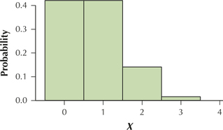
(b) 0 and 1 business major
Question 6.152
54. The binomial experiment in Exercise 50
Question 6.153
55. The binomial experiment in Exercise 51
6.2.55
(a)
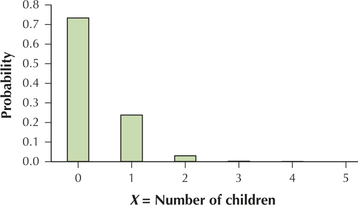
(b) 0 25- to 29-year-olds
Question 6.154
56. The binomial experiment in Exercise 52
APPLYING THE CONCEPTS
Question 6.155
57. Random Guessing on a Quiz. Suppose that you are taking a quiz of five multiple-choice questions (the instructor chose the questions randomly), with each question having four possible responses. You did not study at all for the quiz and will randomly guess the correct response for each question. The random variable is the number of correct responses.
- If each question has four possible responses, why is this a valid binomial experiment?
- State the values of and .
- Calculate the probability that you will pass this quiz by correctly responding to at least three of the five questions. Is this good news for you?
- Use your answer to (c) to find the probability that you will not pass the quiz.
6.2.57
(a) It fulfills the requirements: (i) There are only two possible outcomes for each trial: correct answer or incorrect answer. (ii) We know in advance that the quiz will have 5 questions. (iii) Since you are randomly guessing the answer to each question, the trials are independent. (iv) Since each question has 4 responses, the probability of guessing correctly remains the same from question to question. (b) , (c) 0.1035 (d) 0.8965
Question 6.156
58. Women in Management. According to the U.S. Government Accountability Office, women hold 40% of the management positions in the United States.3 Suppose we take a random sample of 20 people in management positions.
- Find the probability that the sample contains exactly 10 women.
- Find the probability that the sample contains, at most, one woman.
- Find the probability that the sample contains between 8 and 10 women, inclusive.
Question 6.157
59. Abandoning Landlines. The Centers for Disease Control reported in 2014 that 41% of U.S. households use only cell phones (no landline) (Source: http://www.pewresearch.org/fact-tank/2014/07/08/two-of-every-five-u-s-households-have-only-wireless-phones/). Suppose we take a random sample of 12 telephone users.
- Find the probability that the sample contains exactly four users who use cell phones only.
- Find the probability that the sample contains, at most, four users who use cell phones only.
- Find the probability that the sample contains between four and six users inclusive who use cell phones only.
6.2.59
(a) 0.2054 (b) 0.4101 (c) 0.6189
Question 6.158
60. Online Dating. The Pew Research Center reported in 2014 that 22% of 25- to 34-year-olds have used online dating. Suppose we select fifteen 25- to 34-year-olds at random.
- Explain why we cannot use the binomial table to solve probability problems for this binomial experiment.
- Find the probability that the sample contains exactly three 25- to 34-year-olds who have used online dating.
- Find the probability that the sample contains at most three 25- to 34-year-olds who have used online dating.
Question 6.159
61. Random Guessing on a Quiz. Refer to Exercise 57.
- Compute the mean, variance, and standard deviation of . Interpret the mean.
- Use the -score method to determine which numbers of correct responses should be considered outliers.
- Use technology or the binomial table to construct a probability distribution graph of . Then state the mode of , that is, the most likely number of correct responses.
- Find the probability that .
6.2.61
(a) correct answers. If we repeat this experiment an infinite number of times, record the number of correct answers for each quiz taken, and take the mean of all of the quizzes, the mean number of correct answers will equal . correct answer squared, correct answer. (b) Five correct answers is considered an outlier; 4 correct answers is considered moderately unusual. (c) Mode is 1 correct answer.
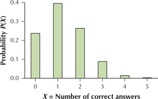
(d) 0.3955
Question 6.160
62. Women in Management. Refer to Exercise 58.
- Find the mean, variance, and standard deviation of the number of women in management positions.
- Suppose that the sample contains six women in management positions. Use the -score method to determine whether this outcome is unusual or not.
- Use technology or the binomial table to determine the most likely number of women in management positions.
- Compute the probability that the sample contains the mode number of women in management positions.
Question 6.161
63. Abandoning Landlines. Refer to Exercise 59.
- Calculate the mean, variance, and standard deviation of the number of users in the sample who have abandoned their landlines. Interpret the mean.
- Suppose the sample contains no users who have abandoned their landlines. Is this outcome unusual or an outlier? Use the -score method to find out.
6.2.63
(a) telephone users who have abandoned their landline; telephone users who have abandoned their landline squared; telephone users who have abandoned their landline. If we take infinitely many random samples of telephone users of size 12 and calculate the mean number of telephone users who have abandoned their landline it would be 4.92. (b) Moderately unusual
Question 6.162
64. Online Dating. Refer to Exercise 60.
- Find the mean, variance, and standard deviation of the number of 25- to 34-year-olds who have used online dating.
- Suppose that the sample contains eight 25- to 34-year-olds who have used online dating. Use the -score method to determine whether this outcome is unusual or not.
Question 6.163
65. Women and Depression. According to the National Institute of Mental Health, nearly twice the proportion of women (12%) as men (6.6%) are affected by a depressive disorder each year. Suppose that random samples of five women and five men are taken. Let represent the number of women affected by a depressive disorder.
- Find and interpret the mean of .
- If possible, find the probability that equals the mean. If not possible, explain why it is not possible to do so.
- Construct the probability distribution graph of , and identify the mode of .
- Find the probability that equals the mode of .
6.2.65
(a) woman. If we repeat this experiment an infinite number of times, record the number of women affected by a depressive disorder for each sample, and take the mean of all the samples, the mean number of women living with a depressive disorder will equal . (b) Not possible. The expected value of is not an integer. (c) women
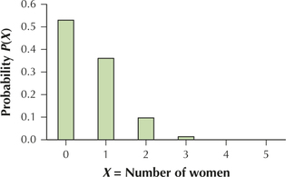
(d) 0.5277
Question 6.164
66. Men and Depression. Refer to Exercise 65. Let represent the number of men affected by a depressive disorder in a random sample of size 5.
- Find and interpret the mean of .
- If possible, find the probability that equals the mean. If not possible, explain why it is not possible to do so.
- Construct the probability distribution graph of , and identify the mode of .
- Find the probability that equals the mode of .
Question 6.165
67. Mean, Median, Mode. For a binomial distribution, if the mean is a whole number, then . Use this equation to answer the following questions:
- Find the median of for the binomial distribution in Example 19.
- Find the mode of for the binomial distribution in Example 19.
- What is the most likely value of for the binomial distribution in Example 19?
6.2.67
(a) 90 students (b) 90 students (c) 90 students
Question 6.166
68. Geometric Probability Distribution. Refer to Example 14(a), where a fisherman is going fishing and will continue to fish until he catches a rainbow trout. This is an example of the geometric probability distribution, which has the same requirements as the binomial distribution, except that there is not a fixed number of trials . Instead, the geometric random variable represents the number of trials until a success is observed. The geometric probability distribution formula is
where represents the probability of success. The possible values of are . The U.S. Census Bureau reported in 2010 that 30% of U.S. households have no access at all to the Internet. A random sample is taken of U.S. households. Let the random variable represent the number of trials until a household is found that has access to the Internet.
- Find the probability that , that is, the first household sampled has access to the Internet.
- Find the probability that , that is, the first household sampled does not have access, but the second household sampled does have access to the Internet.
- Find the probability that , that is, the first two households sampled do not have access, but the third household sampled does have access to the Internet.
Question 6.167
69. Hypergeometric Probability Distribution. If samples are drawn from a relatively small finite population, and the sample size is larger than 1% of the population, so that the 1% Guideline (page 282) does not apply, we should not use the binomial distribution because the samples are not independent. Instead, if we are sampling without replacement, and there are two mutually exclusive categories, then you should use the hypergeometric probability distribution. Suppose that objects belong to the first category (“successes”), and objects belong to the second category (“failures”). Then the probability of getting successes and failures is given by the hypergeometric probability distribution formula:
where , is the population size, and is the sample size. You are dealt 5 cards at random from a deck of 52 cards.
- Find the probability that all 5 cards are spades.
- Find the probability that exactly 4 cards are spades.
- Find the probability that at least 4 cards are spades.
- Find the probability that exactly 3 cards are spades.
- Find the probability that, at most, 2 cards are spades.
6.2.69
(a) (b) (c) (d) (e)
Question 6.168
70. Multinomial Distribution. The multinomial probability distribution is similar to the binomial distribution, except that the binomial involves only two categories, whereas the multinomial involves more than two categories. Suppose we have three mutually exclusive outcomes, , and , where , , and . If we have a sample of independent trials, then the probability that we get outcomes of category , outcomes of category , and outcomes of category is given by the following formula:
Suppose that 30% of students on a particular college campus are Democrats, 30% are Republicans, and 40% are Independents. Suppose we take a random sample of 10 students.
- Find the probability that 3 are Democrat, 3 are Republican, and 4 are Independent.
- Find the probability that 3 are Democrat, 4 are Republican, and 3 are Independent.
- Find the probability that 4 are Democrat, 3 are Republican, and 3 are Independent.
BRINGING IT ALL TOGETHER
Small Business Jobs. According to the U.S. Small Business Administration, small businesses provide 75% of the net new jobs added to the economy. Consider a random sample of 10 new jobs. Let represent the number of the new jobs added to the economy that are provided by small businesses. Use this information for Exercises 71–79.
Question 6.169
71. Confirm that this situation represents a binomial experiment.
6.2.71
(i) Either a new job is provided by a small company or it is not provided by a small company. These are the only two possible outcomes and they are mutually exclusive.
(ii) It is known in advance that exactly 10 new jobs will be selected.
(iii) The sample is random, so the outcomes are independent.
(iv) The sample is quite small compared to the size of the population, so that the probability that a new job was provided by a small business remains the same from job to job.
Question 6.170
72. Use the binomial distribution formula to find the following probabilities:
- That 7 new jobs are provided by small businesses
- That 8 new jobs are provided by small businesses
Question 6.171
73. Use the binomial tables or technology to find the following probabilities. Then explain why the probabilities in (a) and (b) are equal, as are the probabilities in (c) and (d).
6.2.73
(a) 0.2440 (b) 0.2440 (c) 0.0197 (d) 0.0197; is a discrete variable.
Question 6.172
74. Find the following parameters of the binomial distribution for this experiment. Interpret the mean and standard deviation.
- Mean
- Variance
- Standard deviation
Question 6.173
75. If possible, find the probability that equals . If not possible, explain why it is not possible to do so.
6.2.75
Not possible because jobs is not a whole number.
Question 6.174
76. Construct the probability distribution graph of .
Question 6.175
77. Identify the mode of .
6.2.77
8 jobs
Question 6.176
78. Find the probability that equals the mode of .
Question 6.177
79. Following Example 19(c), identify all values of this binomial distribution that are unusual or somewhat unusual.
6.2.79
0, 1, 2, and 3 jobs are outliers. 4 jobs is moderately unusual.
WORKING WITH LARGE DATA SETS
Motor Vehicle Fuel Efficiency. Open the data set FuelEfficiency. We will explore some characteristics of this data set, using the tools and techniques we have learned in this section. Use technology to do Exercises 80–84.
Question 6.178
fuelefficiency
80. Examine the variable class. Make this into a binomial random variable as follows: Consider all vehicles that are compact cars to be a success, and all other vehicles to be a failure. If we use all 1141 vehicles, what is the probability of success?
Question 6.179
fuelefficiency
81. If we take a random sample of 100 vehicles, what is the expected number of compact cars?
6.2.81
16.39 cars
Question 6.180
fuelefficiency
82. If we take a random sample of 100 vehicles, what is the standard deviation of the number of compact cars?
Question 6.181
fuelefficiency
83. Use technology to obtain a random sample of 100 vehicles. How many compact cars are in the sample?
6.2.83
Answers will vary
Question 6.182
fuelefficiency
84. Use the population mean and standard deviation from Exercises 81 and 82 to determine whether the observed number of compact cars in your sample in Exercise 83 is unusual, using the -score method.