7 Sampling Distributions

7.4 Section 7.2 Exercises

CLARIFYING THE CONCEPTS

Question 7.127

1. Explain what a sample proportion is, using as an example the courses for which you got an A last semester. (p. 415)

7.2.1

If we take a sample of size $n$ , the sample proportion $\hat{p}$ is $\hat{p} = x / n$ , where $x$ represents the number of individuals in the sample that have the particular characteristic. Examples will vary.

Question 7.128

2. What is the mean of the sampling distribution of $\hat{p}$ ? (p. 416)

Question 7.129

3. Give the formula for the standard error of the proportion. (p. 416)

7.2.3

$σ_{\hat{p}} = \sqrt{p \cdot (1 - p) / n}$

Question 7.130

4. What are the requirements for the sampling distribution of $\hat{p}$ to be approximately normal? (p. 417)

Question 7.131

5. Suppose you double the sample size. What happens to the standard error of the proportion? (p. 416)

7.2.5

It decreases by a factor of $1 / \sqrt{2} \approx 0.7071$ .

Question 7.132

6. For the following values of $X$ and $n$ , calculate the sample proportion $\hat{p}$ : (p. 415)

$X = 10$ , $n = 40$
$X = 25$ , $n = 75$
$Number of successes = 27$ , $number of trials = 54$
$Number of successes = 1000$ , $number of trails = 1 million$

PRACTICING THE TECHNIQUES

CHECK IT OUT!

To do	Check out	Topic
Exercises 7–18	Example 12	Determining whether the CLT for Proportions applies
Exercises 19–24	Example 13	Minimum sample size for approximating normality
Exercises 25–32	Example 14	Finding probabilities using the CLT for Proportions
Exercises 33–38	Example 15	Finding percentiles using the CLT for Proportions

In Exercises 7–18, samples are taken. Find (a) $μ_{\hat{p}}$ and (b) $σ_{\hat{p}}$ , and (c) determine whether the sampling distribution of $\hat{p}$ is approximately normal or unknown.

Page 422

Question 7.133

7. $p = 0.5$ , $n = 400$

7.2.7

(a) 0.5 (b) 0.025 (c) Approximately normal

Question 7.134

8. $p = 0.5$ , $n = 20$

Question 7.135

9. $p = 0.05$ , $n = 200$

7.2.9

(a) 0.05 (b) 0.01541 (c) Approximately normal

Question 7.136

10. $p = 0.05$ , $n = 100$

Question 7.137

11. $p = 0.3$ , $n = 12$

7.2.11

(a) 0.3 (b) 0.1323 (c) Unknown

Question 7.138

12. $p = 0.3$ , $n = 20$

Question 7.139

13. $p = 0.002$ , $n = 2000$

7.2.13

(a) 0.002 (b) 0.000999 (c) Unknown

Question 7.140

14. $p = 0.002$ , $n = 2500$

Question 7.141

15. $p = 0.02$ , $n = 250$

7.2.15

(a) 0.02 (b) 0.008854 (c) Approximately normal

Question 7.142

16. $p = 0.02$ , $n = 200$

Question 7.143

17. $p = 0.01$ , $n = 500$

7.2.17

(a) 0.01 (b) 0.004450 (c) Approximately normal

Question 7.144

18. $p = 0.01$ , $n = 100$

In Exercises 19–24, find the minimum sample size that produces a sampling distribution of $\hat{p}$ that is approximately normal.

Question 7.145

19. $p = 0.8$

7.2.19

Question 7.146

20. $p = 0.85$

Question 7.147

21. $p = 0.9$

7.2.21

Question 7.148

22. $p = 0.95$

Question 7.149

23. $p = 0.99$

7.2.23

500

Question 7.150

24. $p = 0.999$

For Exercises 25–32, if possible, find the indicated probability. If it is not possible, explain why not.

Question 7.151

25. $p = 0.5$ , $n = 225$ , $P (\hat{p} > 0.55)$

7.2.25

0.0668

Question 7.152

26. $p = 0.5$ , $n = 8$ , $P (\hat{p} > 0.55)$

Question 7.153

27. $p = 0.03$ , $n = 36$ , $P (\hat{p} > 0.011)$

7.2.27

Not possible since $n \cdot p = (36) (0.03) = 1.08 < 5$ .

Question 7.154

28. $p = 0.03$ , $n = 225$ , $P (\hat{p} > 0.011)$

Question 7.155

29. $p = 0.8$ , $n = 50$ , $P (0.88 < \hat{p} < 0.91)$

7.2.29

0.0531

Question 7.156

30. $p = 0.8$ , $n = 81$ , $P (0.88 < \hat{p} < 0.91)$

Question 7.157

31. $p = 0.98$ , $n = 225$ , $P (\hat{p} > 0.981)$

7.2.31

Not possible since $n \cdot q = (225) (0.02) = 4.50 < 5$ .

Question 7.158

32. $p = 0.98$ , $n = 256$ , $P (\hat{p} > 0.981)$

For Exercises 33–38, find the indicated value of $\hat{p}$ . If it is not possible, explain why not.

Question 7.159

33. $p = 0.6$ , $n = 100$ , value of $\hat{p}$ larger than 90% of all values of $\hat{p}$

7.2.33

0.6628

Question 7.160

34. $p = 0.6$ , $n = 100$ , value of $\hat{p}$ larger than 10% of all values of $\hat{p}$

Question 7.161

35. $p = 0.99$ , $n = 225$ , 95th percentile of values of $\hat{p}$

7.2.35

Not possible since $n \cdot q = (225) (0.01) = 2.25 < 5$ .

Question 7.162

36. $p = 0.99$ , $n = 225$ , 5th percentile of values of $\hat{p}$

Question 7.163

37. $p = 0.2$ , $n = 225$ , 2.5th percentile of values of $\hat{p}$

7.2.37

0.1477

Question 7.164

38. $p = 0.2$ , $n = 225$ , 97.5th percentile of values of $\hat{p}$

APPLYING THE CONCEPTS

Question 7.165

39. Abandoning Landlines. The National Health Interview Survey reports that 25% of telephone users no longer use landlines, and have switched completely to cell phone use. Suppose we take samples of size 36.

Find the mean and standard error of the sampling distribution of $\hat{p}$ , the sample proportion of telephone users who no longer use landlines.
Describe the sampling distribution of $\hat{p}$ .
Compute the probability that $\hat{p}$ exceeds 0.26.

7.2.39

(a) $μ_{\hat{p}} = 0.25, σ_{\hat{p}} \approx 0.0722$ (b) Approximately normal (0.25, 0.0722) (c) 0.4443 (TI-83/84: 0.4449)

Question 7.166

40. LeBron James. During the 2013-2014 National Basketball Association season, 75% of LeBron James's free throws were successful. Suppose we take a sample of 50 of LeBron's free throws.

Find $μ_{\hat{p}}$ and $σ_{\hat{p}}$ for the sample proportion of LeBron's free throws that were good.
Describe the sampling distribution of $\hat{p}$ .
Calculate $P (\hat{p} > 0.60)$ .

Question 7.167

41. Small Business Jobs. According to the U.S. Small Business Administration, small businesses provide 75% of the new jobs added to the economy. Suppose we take samples of 20 new jobs.

Find $μ_{\hat{p}}$ and $σ_{\hat{p}}$ for the sample proportion of new jobs added to the economy that are provided by small businesses.
Calculate $P (\hat{p} > 0.69)$ .
Compute $P (0.775 < \hat{p} < 0.8)$ .

7.2.41

(a) $μ_{\hat{p}} = 0.75, σ_{\hat{p}} \approx 0.0968$ (b) 0.7324 (TI-83/84: 0.7323) (c) 0.0959 (TI-83/84: 0.0954)

Question 7.168

42. Facebook Accounts. In 2014, the Harvard University Institute of Politics surveyed 3058 people 18 to 29 years old and found 2569 who had a Facebook account.⁷ Suppose we take samples of 256 18- to 29-year-olds.

Find $μ_{\hat{p}}$ and $σ_{\hat{p}}$ for the sample proportion of 18- to 29-year-olds with Facebook accounts.
Calculate $P (\hat{p} > 0.86)$ .
Compute $P (0.82 < \hat{p} < 0.86)$ .

Question 7.169

43. Abandoning Landlines. Refer to Exercise 39.

Find the 5th and 95th percentiles of the sample proportions.
Draw a graph showing the sampling distribution of $\hat{p}$ , centered at $p$ , with the 5th and 95th percentiles, and the area of 0.90 under the curve between them shaded.
Suppose only 2 of 36 phone users in a sample abandoned their landlines. Would this be considered an outlier? Explain your reasoning. (Hint: Use the Z-score method.)
Determine which sample proportions would be considered outliers.

7.2.43

(a) 0.1312, 0.3688

(b)

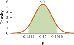
(c) For $\hat{p} = 2 / 36 \approx 0.0556, Z = - 2.69$ . Thus $\hat{p} = 2 / 36$ is considered moderately unusual. (d) Sample proportions between 0 and 0.0334 inclusive and between 0.4666 and 1 inclusive would be considered outliers.

Question 7.170

44. LeBron James. Refer to Exercise 40.

Find the 2.5th and 97.5th percentiles of the sample proportions.
Draw a graph showing the sampling distribution of $\hat{p}$ , centered at $p$ , with the 2.5th and 97.5th percentiles, and the area of 0.95 under the curve between them shaded.
In the May 20, 2014 playoff game against the Indiana Pacers, LeBron James had only a 50% success rate from the free-throw line. Would that be considered “poor shooting” by his standards? Explain your reasoning. (Hint: Use the Z-score method.)
Later in the same series, in the May 30, 2014 playoff game against the Indiana Pacers, LeBron James had a perfect 100% success rate from the free-throw line. Would that be considered “hot shooting” by his standards? Explain your reasoning.

Question 7.171

45. Small Business Jobs. Refer to Exercise 41.

Find the 0.5th and 99.5th percentiles of the sample proportions.
Page 423
Draw a graph showing the sampling distribution of $\hat{p}$ , with the area between the 0.5th and 99.5th percentiles shaded.
Suppose 14 of 20 new jobs added to the economy were provided by small business. Would this be considered unusual? Explain your reasoning.

7.2.45

(a) 0.5003, 0.9997 (TI-83/84: 0.5007, 0.9993)

(b)

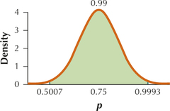
(c) For $\hat{p} = 14 / 20 = 0.7, Z = - 0.5165$ . Thus $\hat{p} = 0.7$ is neither moderately unusual nor an outlier.

Question 7.172

46. Facebook Accounts. Refer to Exercise 42.

Find the 2.5th and 97.5th percentiles of the sample proportions.
Draw a graph showing the sampling distribution of $\hat{p}$ , with the area between the 2.5th and 97.5th percentiles shaded.
Calculate $P (\hat{p} < 0.82)$ .
Suppose someone claimed that the proportion of all 18- to 29-year-olds who had a Facebook account was less than 0.82. Based on the probability you calculated in (c), do you think there is strong evidence against this claim?

Question 7.173

47. Facebook Accounts. Refer to Exercises 42 and 46. What if we increased the sample size to some unspecified larger number? Describe how and why the following quantities would change, if at all:

$μ_{\hat{p}}$
$σ_{\hat{p}}$
$P (\hat{p} > 0.86)$
$P (0.82 < \hat{p} < 0.86)$
$P (\hat{p} < 0.82)$
2.5th percentile of the sample proportions
97.5th percentile of the sample proportions

7.2.47

(a) Remains the same since $μ_{\hat{p}} = p$ does not depend on $n$ .

(b) Decrease. Since the sample size $n$ is in the denominator of $σ_{\hat{p}} = \sqrt{\frac{p \cdot q}{n}}, σ_{\hat{p}}$ decreases as the sample size $n$ increases. (c) Decrease. Standardizing we get $Z = \frac{0.86 - μ_{\hat{p}}}{σ_{\hat{p}}} = \frac{0.86 - 0.840}{σ_{\hat{p}}} = \frac{0.02}{σ_{\hat{p}}}$ . From (b), $σ_{\hat{p}}$ decreases as the sample size $n$ increases. Therefore $Z = \frac{0.02}{σ_{\hat{p}}}$ increases as the sample size $n$ increases. Therefore $P (\hat{p} > 0.86) = P (Z > \frac{0.02}{σ_{\hat{p}}})$ decreases.

(d) Increase. Standardizing we get $Z = \frac{0.82 - μ_{\hat{p}}}{σ_{\hat{p}}} = \frac{0.82 - 0.840}{σ_{\hat{p}}} = \frac{- 0.02}{σ_{\hat{p}}}$ and $Z = \frac{0.86 - μ_{\hat{p}}}{σ_{\hat{p}}} = \frac{0.86 - 0.840}{σ_{\hat{p}}} = \frac{0.02}{σ_{\hat{p}}}$ . From (b), $σ_{\hat{p}}$ decreases as the sample size $n$ increases. Therefore $Z = \frac{- 0.02}{σ_{\hat{p}}}$ decreases and $Z = \frac{0.02}{σ_{\hat{p}}}$ increases as the sample size $n$ increases. Thus $P (0.82 < \hat{p} < 0.86) = P (\frac{- 0.02}{σ_{\hat{p}}} < Z < \frac{0.02}{σ_{\hat{p}}})$ increases as the sample size $n$ increases. (e) Decrease. Standardizing we get $Z = \frac{0.82 - μ_{\hat{p}}}{σ_{\hat{p}}} = \frac{0.82 - 0.840}{σ_{\hat{p}}} = \frac{- 0.02}{σ_{\hat{p}}}$ . From (b), $σ_{\hat{p}}$ decreases as the sample size $n$ increases. Therefore $Z = \frac{- 0.02}{σ_{\hat{p}}}$ decreases as the sample size $n$ increases. Thus $P (\hat{p} < 0.82) = P (Z < \frac{- 0.02}{σ_{\hat{p}}})$ decreases as the sample size $n$ increases. (f) Increase. The 2.5th percentile is found by the formula ${\hat{p}}_{1} = (- 1.96) σ_{\hat{p}} + μ_{\hat{p}}$ . From (a) $μ_{\hat{p}}$ remains the same as the sample size $n$ increases and from (b) $σ_{\hat{p}}$ decreases as the sample size $n$ increases. Therefore ${\hat{p}}_{1} = (- 1.96) σ_{\hat{p}} + μ_{\hat{p}}$ increases as the sample size $n$ increases. (g) Decrease. The 97.5th percentile is found by the formula ${\hat{p}}_{2} = (- 1.96) σ_{\hat{p}} + μ_{\hat{p}}$ . From (a) $μ_{\hat{p}}$ remains the same as the sample size $n$ increases and from (b), $σ_{\hat{p}}$ decreases as the sample size $n$ increases. Therefore ${\hat{p}}_{2} = (- 1.96) σ_{\hat{p}} + μ_{\hat{p}}$ decreases as the sample size $n$ increases.

BRINGING IT ALL TOGETHER

Partners Checking Up on Each Other. Use the following information for Exercises 48–51. According to a study in the journal Computers in Human Behavior,⁸ 65% of the college women surveyed checked the call histories on the cell phones of their partners, whereas 41% of the males did so.

Question 7.174

48. Suppose we take a sample of 100 college females and 100 college males.

Find $μ_{\hat{p}}$ and $σ_{\hat{p}}$ for the sample proportion of females checking the call histories of their partners.
Find $μ_{\hat{p}}$ and $σ_{\hat{p}}$ for the sample proportion of males checking the call histories of their partners.

Question 7.175

49. Refer to Exercise 48. Calculate the following probabilities:

That more than 65% of the females checked the call histories of their partners
That more than 65% of the males checked the call histories of their partners
That less than 41% of the females checked the call histories of their partners
That less than 41% of the males checked the call histories of their partners

7.2.49

(a) 0.5 (b) 0 (c) 0 (d) 0.5

Question 7.176

50. Refer to Exercise 48.

Find the 2.5th and 97.5th percentiles of the sample proportions of females checking the call histories of their partners.
Find the 2.5th and 97.5th percentiles of the sample proportions of males checking the call histories of their partners.

Question 7.177

51. Suppose someone claimed that there really was no difference in the proportions of females and males who check the call histories on their partners' cell phones. How would you use the results from Exercises 49 and 50 to address this claim?

7.2.51

The results of Exercises 49 and 50 do not support this claim. The 97.5th percentile for the males is less than the 2.5th percentile for the females. Also $P (p < 0.41)$ and $P (p > 0.65)$ are both very different for males and females.