8 Confidence Intervals

8.3 $Z$ Interval for the Population Proportion

This page includes Video Technology Manuals

OBJECTIVES By the end of this section, I will be able to …

Calculate the point estimate $\hat{p}$ of the population proportion $p$ .
Construct and interpret a $Z$ interval for the population proportion $p$ .
Compute and interpret the margin of error for the $Z$ interval for $p$ .
Determine the sample size needed to estimate the population proportion.

1 Point Estimate $\hat{p}$ of the Population Proportion $p$

So far, we have dealt with interval estimates of the population mean $μ$ only. However, we may also be interested in an interval estimate for the population proportion of successes, $p$ . Recall from Section 7.2 that the sample proportion of successes

$\hat{p} = \frac{x}{n} = \frac{number of successes}{sample size}$

is a point estimate of the population proportion $p$ .

EXAMPLE 17 Point estimate $\hat{p}$ of the population proportion $p$

Suppose that a random sample of 100 Starbucks' sales transactions is taken, and that 10 of these transactions were made using a cell phone. Calculate the sample proportion $\hat{p}$ , and use it as a point estimate of the population proportion $p$ .

Solution

We have $n = 100$ transactions and $x = 10$ . Thus,

$\hat{p} = \frac{x}{n} = \frac{10}{100} = 0.1$

The point estimate of the population proportion $p$ of Starbucks' transactions made using a cell phone is 0.1. (This sample proportion of 0.1 reflects the results from a survey made by the Wall Street Journal in 2013.¹⁶)

NOW YOU CAN DO

Exercises 3–6.

YOUR TURN#11

For the following values of $n$ and $x$ , calculate the sample proportion $\hat{p}$ , and use it as a point estimate of the population proportion $p$ .

$n = 100$ , $x = 50$
$n = 160$ , $x = 90$

(The solutions are shown in Appendix A.)

Of course, different samples of Starbucks' customers may turn up different sample proportions $\hat{p}$ . These are point estimates, and thus they carry no measure of confidence in their accuracy. The point estimates are probably close to the true values, but it's possible that they are not. They may be far from the true values. Only by using confidence intervals can we make probability statements about the accuracy of the estimates.

Page 464

2 $Z$ Interval for the Population Proportion $p$

Alternatively, the conditions may be expressed as follows: $x \geq 5$ and $(n - x) \geq 5$ , that is, the number of successes ≥5 and the number of failures ≥5. Feel free to use these alternative conditions when the calculations are easier.

Recall the Central Limit Theorem for Proportions in Section 7.2.

Central Limit Theorem for Proportions

The sampling distribution of the sample proportion $\hat{p}$ follows an approximately normal distribution with mean $μ_{\hat{p}} = p$ and standard deviation $σ_{\hat{p}} = \sqrt{\frac{p \cdot q}{n}}$ when both the following conditions are satisfied: (1) $n \cdot p \geq 5$ and (2) $n \cdot q \geq 5$ , where $q = 1 — p$ .

We can use the Central Limit Theorem for Proportions to construct confidence intervals for the population proportion $p$ . Because the confidence interval for $p$ is based on the standard normal $Z$ distribution, it is called the $Z$ interval for the population proportion $p$ . Because $p$ is unknown, the conditions and the formula for $σ_{\hat{p}}$ substitute $\hat{p}$ for $p$ .

$Z$ Interval for $p$

The $Z$ interval for $p$ may be performed only if both the following conditions are met: $n \cdot \hat{p} \geq 5$ and $n \cdot \hat{q} \geq 5$ (alternatively, $x \geq 5$ and $(n - x) \geq 5$ ) where $\hat{q} = 1 - \hat{p}$ . When a random sample of size n is taken from a binomial population with unknown population proportion $p$ , the $100 (1 - α) %$ confidence interval for $p$ is given by

$\begin{array}{l} lower bound = \hat{p} - Z_{α / 2} \sqrt{\frac{\hat{p} \cdot \hat{q}}{n}} \\ upper bound = \hat{p} + Z_{α / 2} \sqrt{\frac{\hat{p} \cdot \hat{q}}{n}} \end{array}$

Alternatively,

$\hat{p} \pm Z_{α / 2} \sqrt{\frac{\hat{p} \cdot \hat{q}}{n}}$

where $\hat{p}$ is the sample proportion of successes, $\hat{q} = 1 - \hat{p}$ , $n$ is the sample size, and $Z_{α / 2}$ depends on the confidence level.

For convenience, we repeat Table 1 here, showing the $Z_{α / 2}$ values for the most common confidence levels.

Table 8.26: Table 1

$Z_{α / 2}$ values for common confidence levels

Confidence level	$α$	$α / 2$	$Z_{α / 2}$
80%	0.20	0.10	1.28
90%	0.10	0.05	1.645
95%	0.05	0.025	1.96
99%	0.01	0.005	2.576

EXAMPLE 18 $Z$ interval for the population proportion $p$

Using the Starbucks' data from Example 17, (a) verify that the conditions for constructing the $Z$ interval for $p$ have been met, and (b) construct a 95% confidence interval for the population proportion of all Starbucks' transactions that are made using a cell phone.

Page 465

Solution

We have $n = 100$ transactions and $x = 10$ . We check the conditions for the confidence interval. There are $x = 10$ successes, which is ≥5, and there are $n - x = 90$ failures, which is also ≥5. The conditions for constructing the $Z$ interval for $p$ have been met.
From Table 1, the confidence level of 95% gives $Z_{α / 2} = 1.96$ . Thus, the confidence interval is
$\begin{array}{l} lower bound & = \hat{p} - Z_{α / 2} \sqrt{\frac{\hat{p} \cdot \hat{q}}{n}} = 0.1 - 1.96 \sqrt{\frac{0.1 (0.9)}{100}} \\ = 0.1 - 1.96 (0.03) = 0.1 - 0.0588 = 0.0412 \\ upper bound & = \hat{p} + Z_{α / 2} \sqrt{\frac{\hat{p} \cdot \hat{q}}{n}} = 0.1 + 1.96 \sqrt{\frac{0.1 (0.9)}{100}} \\ = 0.1 + 1.96 (0.03) = 0.1 + 0.0588 = 0.1588 \end{array}$

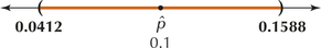
We are 95% confident that the population proportion of Starbucks' sales transactions made using a cell phone lies between 0.0412 and 0.1588. (See Figure 27.)

FIGURE 27 95% Confidence interval for the population proportion of Starbucks' sales transactions made using a cell phone.

NOW YOU CAN DO

Exercises 7–20.

YOUR TURN#12

For the following values of $n$ and $x$ , (i) confirm that the conditions have been met, and (ii) construct a 95% confidence interval for the population proportion $p$ .

$n = 100$ , $x = 50$
$n = 160$ , $x = 90$

(The solutions are shown in Appendix A.)

EXAMPLE 19 $Z$ intervals for $p$ using technology

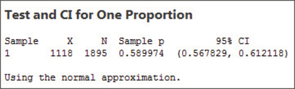
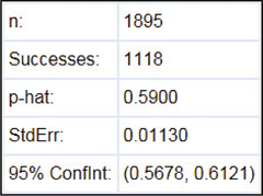
A Pew Research Center survey of 1895 Internet users found 1118 who agree that “online dating is a good way to meet people.” Use technology to find a 95% confidence interval for the population proportion of all Internet users who agree that online dating is a good way to meet people.

Solution

We use the instructions provided in the Step-by-Step Technology Guide at the end of this section (page 469). The results for the TI-83/84 in Figure 28 display the 95% confidence interval for the population proportion of Americans who agree that online dating is a good way to meet people to be

$(lower bound = 0.56783, upper bound = 0.61212)$

FIGURE 28 TI-83/84 results.

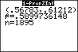
They also show the sample proportion $\hat{p} = 0.5899736148$ and the sample size $n = 1895$ .

Page 466

The results for Minitab are shown in Figure 29. Minitab provides the sample number of successes $X = 1118$ , the sample size $n = 1895$ , the sample proportion $\hat{p} = 0.589974$ , and the 95% confidence interval for $p (0.567829, 0.612118)$ .

FIGURE 29 Minitab results for the

$Z$ interval for

$p$ .

The results for CrunchIt! are shown in Figure 30. CrunchIt! provides the sample size $n = 1895$ , the sample number of successes $X = 1118$ , the sample proportion $\hat{p} = 0.59$ , and the 95% confidence interval for $p (0.5678, 0.6121)$ .

FIGURE 30 CrunchIt! results for the

$Z$ interval for

$p$ .

3 Margin of Error for the $Z$ Interval for $p$

For the $Z$ interval for the population proportion $p$ , the margin of error is given as follows.

Margin of Error for the $Z$ Interval for $p$

$E = Z_{α / 2} \cdot \sqrt{\frac{\hat{p} \cdot \hat{q}}{n}}$

The margin of error $E$ for a $(1 - α) 100 %$ $Z$ interval for $p$ can be interpreted as follows:

“We can estimate the population proportion $p$ to within $E$ with $(1 - α) 100 %$ confidence.”

Note that, just like the confidence interval for $μ$ , the $Z$ interval for $p$ takes the form

$\begin{array}{l} point estimate \pm margin of error \\ \begin{array}{l} = \hat{p} \pm Z_{α / 2} \sqrt{\frac{\hat{p} \cdot \hat{q}}{n}} \\ = \hat{p} \pm E \end{array} \end{array}$

EXAMPLE 20 Margin of error: The famous “plus or minus 3 percentage points”

Hardly a day goes by without some new poll being published. Polls influence the choice of candidates and the direction of their policies, especially during election campaigns. For example, the Gallup Organization polled 1012 American adults, asking them, “Do you think there should or should not be a law that would ban the possession of handguns, except by the police and other authorized persons?” Of the 1012 randomly chosen respondents, 374 said that there should be such a law.

Page 467

Check that the conditions for the $Z$ interval for $p$ have been met.
Find and interpret the margin of error $E$ .
Construct and interpret a 95% confidence interval for the population proportion of all American adults who think there should be such a law.

Solution

The sample size is $n = 1012$ . The observed proportion is $\hat{p} = \frac{374}{1012} \approx 0.37$ , so $\hat{q} = (1 - \hat{p}) = 0.63$

We next check the conditions for the confidence interval. There are $x = 374$ successes and $n - x = 1012 - 374 = 638$ failures. Because neither is less than 5, the conditions are met.
The confidence level of 95% implies that our $Z_{α / 2}$ equals 1.96 (from Table 8.1). Thus, the margin of error equals

$E = Z_{α / 2} \cdot \sqrt{\frac{\hat{p} \cdot \hat{q}}{n}} = 1.96 \cdot \sqrt{\frac{0.37 (0.63)}{1012}} \approx 0.02975 \approx 0.03$

We can estimate the population proportion of all Americans who think that there should be such a law to within $E = 0.03$ with 95% confidence.
The 95% confidence interval is
$\begin{array}{l} \begin{array}{l} point estimate \pm margin of error \\ = \hat{p} \pm Z_{α / 2} \sqrt{\frac{\hat{p} \cdot \hat{q}}{n}} \end{array} \\ = \hat{p} \pm E \\ \approx 0.37 \pm 0.03 \\ = (lower bound = 0.34, upper bound = 0.40) \end{array}$

Note: Here we see the “plus or minus 3 percentage points.”

Thus, we are 95% confident that the population proportion of all American adults who think that there should be such a law lies between 34% and 40%.

NOW YOU CAN DO

Exercises 21–32.

YOUR TURN#13

Refer to Your Turn #12 after Example 18. Find and interpret the margin of error for the following:

Your confidence interval in part (a)
Your confidence interval in part (b)

(The solutions are shown Appendix A.)

Developing Your Statistical Sense

Famous “Plus or Minus 3 Points”

Note that this confidence interval was obtained by adding and subtracting 3% from the 37% point estimate. That is, the poll has a margin of error of $E = 3 percentage points = 0.03$ . This is the famous “plus or minus 3 percentage points” used in many news reports. However, newscasters rarely announce the confidence level of the poll. National pollsters most often use 95% as their confidence level and usually try to select the sample size necessary to create a margin of error of about 3%. We learn how they do this next.

Page 468

4 Sample Size for Estimating the Population Proportion

Next, we consider the question: How large a sample size do I need to estimate the population proportion $p$ to within margin of error $E$ with $100 (1 - α) %$ confidence? The margin of error of the confidence interval for proportions equals

$E = Z_{α / 2} \cdot \sqrt{\frac{\hat{p} \cdot \hat{q}}{n}}$

Solving for $n$ gives us

$\begin{matrix} n = \hat{p} \cdot \hat{q} {(\frac{Z_{α / 2}}{E})}^{2} & (Equation 1) \end{matrix}$

Unfortunately, Equation 1 depends on prior knowledge of $\hat{p}$ . So, if we have such information about $\hat{p}$ available from some earlier sample, then we use Equation 1 to determine the required sample. However, what if we do not know the value of $\hat{p}$ ?

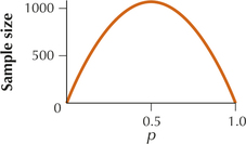
Figure 31 plots the sample size requirements for a 95% confidence interval for $p$ , with a desired margin of error of 0.03, for values of $\hat{p}$ ranging from 0.01 to 0.99, representing all sample proportions from 1% to 99%. Note that the plot is symmetric, and therefore the largest required sample size occurs at the midpoint $\hat{p} = 0.5$ . Thus, $\hat{p} = 0.5$ is the most conservative value for $\hat{p}$ . When the actual value of $\hat{p}$ is not known, we use the following formula:

$n = {(\frac{0.5 \cdot Z_{α / 2}}{E})}^{2}$

FIGURE 31 Sample size required with a margin of error of 0.03 for the range of values

$p$ .

Sample Size for Estimating a Population Proportion

When $\hat{p}$ is known, the sample size needed to estimate the population proportion $p$ to within a margin of error $E$ with confidence $100 (1 - α) %$ is given by

$n = \hat{p} \cdot \hat{q} {(\frac{Z_{α / 2}}{E})}^{2}$

where $Z_{α / 2}$ is the value associated with the desired confidence level, $E$ is the desired margin of error, and $\hat{p}$ is the sample proportion of successes available from some earlier sample and $\hat{q} = 1 - \hat{p}$ Round up to the next integer.

When $\hat{p}$ is unknown, we use

$n = {(\frac{0.5 \cdot Z_{α / 2}}{E})}^{2}$

These formulas are illustrated using the following two examples.

EXAMPLE 21 Sample size for estimating $p$ when $\hat{p}$ is known

Refer to Example 20. Suppose that the Gallup Organization now wanted to estimate the population proportion of those who think there should be a law that would ban the possession of handguns to within a margin of error of $E = 0.01$ with 95% confidence. How large a sample size is needed?

Solution

From Example 20, we have the sample proportion $\hat{p} = 0.37$ . The confidence level of 95% implies that our $Z_{α / 2} = 1.96$ , and the desired margin of error is $E = 0.01$ . Thus, the required sample size is

Page 469

$n = \hat{p} \cdot \hat{q} {(\frac{Z_{α / 2}}{E})}^{2} = 0.37 (0.63) {(\frac{1.96}{0.01})}^{2} \approx 8954.77$

Rounding up, this gives us a minimum required sample size of 8955. The smaller margin of error requires a larger sample size.

NOW YOU CAN DO

Exercises 33–38.

YOUR TURN#14

For the situation in Example 21, suppose Gallup wants the estimate to be within a margin of error of 0.03 with 99% confidence. How large a sample size is needed?

(The solution is shown in Appendix A.)

EXAMPLE 22 Sample size for estimating $p$ when $\hat{p}$ is unknown

Suppose your state wants to take a poll on the proportion of its citizens who support a single statewide primary instead of primaries for each party. No poll on this subject has been taken before, so no prior information is available on the value of the sample proportion, $\hat{p}$ . How large a sample size does the state need to estimate the proportion to within plus or minus 3 percentage points ( $E = 0.03$ ) with 95% confidence?

Solution

The 95% confidence implies that the value for $Z_{α / 2}$ is 1.96. Because no information is available about the value of the population proportion of all state citizens who support a single statewide primary, we use 0.5 as our most conservative value of $p$ :

$n = {[\frac{0.5 \cdot Z_{α / 2}}{E}]}^{2} = {[\frac{(0.5) (1.96)}{0.03}]}^{2} \approx 1067.11$

So if the pollsters want to estimate the population proportion of all state citizens who support a single statewide primary to within 3% with 95% confidence, they will need a sample of 1068 voters (don't forget to round up!).

NOW YOU CAN DO

Exercises 39–46.

YOUR TURN#15

For the scenario in Example 22, suppose the state does not have the funds to contact 1068 voters, and it wants the estimate to be within a margin of error of 0.05 with 95% confidence. How large a sample size is needed?

(The solution is shown in Appendix A.)

8.3 Z<math><mi>Z</mi></math> Interval for the Population Proportion

8.3 $Z$ Interval for the Population Proportion