7.3 7.2 Central Limit Theorem for Proportions
 This page includes Video Technology Manuals
 This page includes Statistical Videos
OBJECTIVES By the end of this section, I will be able to …
- Explain the sampling distribution of the sample proportion ˆp.
- Apply the Central Limit Theorem for Proportions to solve probability questions about the sample proportion.
1 Sampling Distribution of the Sample Proportion ˆp
The sample mean is not the only statistic that can have a sampling distribution. Every sample statistic has a sampling distribution. One of the most important is the sampling distribution of the sample proportion ˆp.
Suppose each individual in a population either has or does not have a particular characteristic. If we take a sample of size n from this population, the sample proportion ˆp (read “p-hat”) is
ˆp=Xn
where X represents the number of individuals in the sample that have the particular characteristic. We use ˆp to estimate the unknown value of the population proportion p.
EXAMPLE 10 Calculating the sample proportion ˆp

In 2014, the Harvard University Institute of Politics surveyed 3058 18- to 29-year-olds and found 1223 who had a Twitter account. Calculate the sample proportion of 18- to 29-year-olds who had a Twitter account.6
Solution
The survey sample size is n=3058, and the number of successes is X=1223. We calculate
ˆp=Xn=12233058=0.4
Thus, the sample proportion of 18- to 29-year-olds who had a Twitter account is 0.4. That is, ˆp=0.4, or 40%, of 18- to 29-year-olds had a Twitter account.
YOUR TURN#6
Refer to Example 10. The same survey found that 1009 had a Pinterest account. Calculate the sample proportion that had a Pinterest account.
(The solution is shown in Appendix A.)
Like ˉx, the sample proportion ˆp varies from sample to sample. And because we do not know its value before taking the sample, ˆp is a random variable. Just as we learned about the Central Limit Theorem for Means in Section 7.1, here in Section 7.2, we develop a Central Limit Theorem for Proportions, where the sampling distribution of the sample proportion becomes approximately normal if the right conditions are satisfied.
The sampling distribution of the sample proportion ˆp for a given sample size n consists of the collection of the sample proportions of all possible samples of size n from the population.
In general, the sampling distribution of any particular statistic for a given sample size n consists of the collection of the values of that sample statistic across all possible samples of size n.
Recall that in Section 7.1, we found that the mean of the sampling distribution of the sample mean ˉx is μˉx=μ and the standard error of the mean is σˉx=σ/√n. We now learn the mean and standard error of the sampling distribution of the sample proportion ˆp.
Fact 5: Mean of the Sampling Distribution of the Sample Proportion ˆp
The mean of the sampling distribution of the sample proportion ˆp is the value of the population proportion p. This may be denoted as μˆp=p and read as “the mean of the sampling distribution of ˆp is p.”
Fact 5 provides a measure of center for the sampling distribution of the sample proportion ˆp, and Fact 6 provides a measure of spread.
Fact 6: Standard Deviation of the Sampling Distribution of the Sample Proportion ˆp
The standard deviation of the sampling distribution of the sample proportion ˆp is σˆp=√p·qn, where p is the population proportion, q=1-p, and n is the sample size. σˆp is called the standard error of the proportion.
EXAMPLE 11 Mean and standard error of ˆp
The National Institutes of Health reported that color blindness linked to the X chromosome afflicts 8% of men. Suppose we take a random sample of 100 men and let p denote the proportion of men in the population who have color blindness linked to the X chromosome. Find μˆp and σˆp.
Solution
First, we note that this is a binomial experiment with p=0.08 and n=100. Fact 5 tells us that μˆp=p; that is, the sampling distribution of the sample proportion ˆp has a mean of p=0.08. Fact 6 states that the standard error is
σˆp=√p·qn=√0.08·(1-0.08)100=√0.000736≈0.02713
YOUR TURN#7
Refer to Example 11. Suppose we take a random sample of 400. Find μˆp and σˆp.
(The solution is shown in Appendix A.)
What Do These Numbers Mean?
Imagine that we repeatedly draw random samples of 100 men and observe the proportion of men ˆp in each sample who have color blindness linked to the X chromosome. Each sample provides us with a value for ˆp. Eventually, the values for ˆp, when graphed, form the sampling distribution shown in Figure 13.
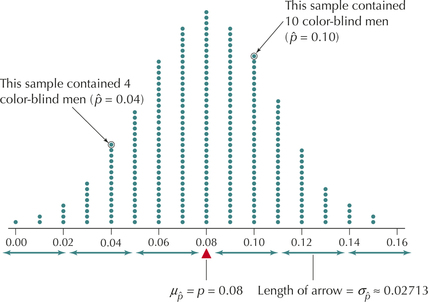
Note that μˆp=p=0.08 is located at the balance point of this distribution, which we should expect because the mean proportion of these samples is μˆp=p=0.08 Each arrow represents 1 standard error σˆp=0.02713. Note that nearly all the sample proportions lie within 3 standard errors of the mean.
Unfortunately, the sampling distribution of ˆp is not always normal. Recall from Section 7.1 that the approximate normality provided by the Central Limit Theorem for Means was a useful tool for solving probability problems for the sample mean ˉx. Similarly, in order to solve probability problems for the sample proportion ˆp, we need a way to achieve approximate normality for the sampling distribution of ˆp. Conditions for the approximate normality of the sampling distribution of ˆp are as follows.
Fact 7: Conditions for Approximate Normality of the Sampling Distribution of the Sample Proportion ˆp
The sampling distribution of the sample proportion ˆp may be considered approximately normal only if both the following conditions hold:
n·p≥5 and n·q≥5
Alternatively, the conditions may be expressed as follows: x≥5 and (n-x)≥5.
The minimum sample size required to produce approximate normality in the sampling distribution of ˆp is the larger of either
n1=5p or n2=5q
(rounded up to the next integer).
2 Applying the Central Limit Theorem for Proportions
Using information from Facts 5, 6, and 7, we express the Central Limit Theorem for Proportions.
Central Limit Theorem for Proportions
The sampling distribution of the sample proportion ˆp follows an approximately normal distribution with mean μˆp=p and standard deviation σˆp=√p·qn when both the following conditions are satisfied: n·p≥5 and n·q≥5.
Alternatively, the conditions may be expressed as follows: x≥5 and (n-x)≥5.
EXAMPLE 12 Determining whether the Central Limit Theorem for Proportions applies
In Example 11, we learned that color blindness linked to the X chromosome afflicts 8% of men. Determine the approximate normality of the sampling distribution of ˆp, the proportion of men who have color blindness linked to the X chromosome, for samples of size (a) 50 and (b) 100.
Solution
We need to check both conditions to find whether the sampling distribution of ˆp is approximately normal.
We are given that p=0.08 and n=50
n·p=50·0.08=4 and n·q=50·(0.92)=46
Because 4 is not ≥ 5, the first condition is not satisfied. The Central Limit Theorem for Proportions cannot be used. We cannot conclude that the sampling distribution of ˆp is approximately normal.
Here, p=0.08 and n=100.
n·p=100·0.08=8 and n·q=100·(0.92)=92
Because both 8 and 92 are ≥ 5, both conditions are satisfied. The Central Limit Theorem for Proportions applies, and we can conclude that the sampling distribution of ˆp is approximately normal. From Example 11, we have μˆp=0.08 and σˆp=0.02713. Thus, the sampling distribution of ˆp is approximately normal with μˆp=0.08 and σˆp=0.02713
NOW YOU CAN DO
Exercises 7–18.
EXAMPLE 13 Minimum sample size for approximate normality
According to George Washington University, 4.3% of all vehicles on the road are large trucks. Let p=0.043 represent the population proportion.
- Find the minimum size of the samples that produces a sampling distribution of ˆp that is approximately normal.
- Describe the sampling distribution of ˆp if we use this minimum sample size.
Solution
Using Fact 7, the minimum sample size required is the larger of either
n1=5p or n2=5q
Here,
n1=5p=50.043≈116.3 and n2=5q=50.957≈5.2
Page 419The larger of n1 and n2 is n1=116.3. However, it is unclear what “0.3” of a vehicle means. So we round up to the next integer: n=117. Therefore, the minimum sample size required to produce a sampling distribution of ˆp that is approximately normal is n=117 vehicles. We confirm that this satisfies our conditions:
n·p=(117)(0.043)=5.031≥5 and n·q=(117)(0.957)=111.969≥5
We have μˆp=0.043 and
σˆp=√pqn=√0.043(0.957)117≈√0.00035172≈0.01875
Because the conditions are met, the Central Limit Theorem for Proportions applies. The sampling distribution of ˆp is approximately normal (μˆp=0.043,σˆp=0.01875).
NOW YOU CAN DO
Exercises 19–24
In those cases where we determine that the sampling distribution of ˆp is approximately normal, we can standardize using Fact 8 to obtain the standard normal Z. Then we may proceed to apply the normal distribution methods we learned in Chapter 6. Fact 8 for proportions is similar to Fact 4 for means.
Fact 8: Standardizing a Normal Sampling Distribution for Proportions
When the sampling distribution of ˆp is approximately normal, we can standardize to produce the standard normal Z:
Z=ˆp-μˆpσˆp=ˆp-p√pqn
where p is the population proportion of successes, q=1-p, and n is the sample size.
EXAMPLE 14 Finding probabilities Using the Central Limit Theorem for Proportions
Using the information in Example 13, find the probability that a sample of vehicles will have a proportion of large trucks greater than 9% for samples of size (a) 30 vehicles and (b) 117 vehicles.
Solution
- We found in Example 13(a) that this sample size of n=30 does not meet the minimum sample size required for the sampling distribution of ˆp to be approximately normal, so we cannot conclude that the sampling distribution of ˆp is approximately normal. Thus, we cannot solve this problem.
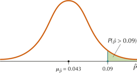
From Example 13(b), the sampling distribution of ˆp is approximately normal with mean μˆp=0.043 and standard deviation σˆp=0.01875. We are then faced with a normal probability problem similar to those in Section 6.5. Figure 14 shows the sampling distribution of ˆp and the probability we are interested in, P(ˆp>0.09). Using Fact 8, we standardize as follows:
Z=0.09-μˆpσˆp=0.09-0.0430.01875≈2.51
Thus, P(ˆp>0.09)=P(Z>2.51), as shown in Figure 15.
Again, we can use our normal distribution methods from Section 6.5 because the Central Limit Theorem for Proportions gives us approximate normality.
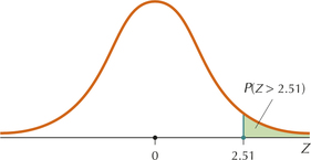
Following Table 8 in Chapter 6 (page 355), we look up Z=2.51 in the Z table and subtract this table area (0.9940) from 1 to get the desired tail area. That is,
P(Z>2.51)=1-0.9940=0.006
So the probability that the sample proportion of large trucks will exceed 0.09 is 0.006.
NOW YOU CAN DO
Exercises 25–32.
YOUR TURN#8
Using the information in Example 13, find the probability that a sample of vehicles will have a proportion of large trucks smaller than 4% for a sample of size n=225 vehicles.
(The solution is shown in Appendix A.)
EXAMPLE 15 Finding percentiles Using the Central Limit Theorem for Proportions
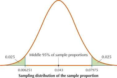
Using the information from Example 13, find the 2.5th and the 97.5th percentiles of sample proportions for n=117.
Solution
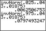
We use the inverse normal function on the TI-83/84, just as we did in Example 8 (page 406). The results, using mean μˆp=0.043 and standard deviation σˆp=0.01875, are shown in Figure 16. We have the 2.5th percentile ≈0.006251 and the 97.5th percentile ≈0.079475.
The 2.5th and the 97.5th percentiles contain the middle 95% of sample proportions, as shown in Figure 17.
NOW YOU CAN DO
Exercises 33–38.
YOUR TURN#9
Using the information from Example 13, find the two percentiles that contain the middle 90% of sample proportions.
(The solution is shown in Appendix A.)
Developing Your Statistical Sense
Pitfalls of Using an Approximation
Let's use symmetry and the results from Example 15 to find the 1st percentile of the sampling distribution of ˆp for n=117. By symmetry, the 1st percentile will be the same distance below the mean that the 99th percentile is above the mean. The 99th percentile, 0.0867, lies (0.0867-0.043)=0.0437 above the mean. Therefore, the 1st percentile lies 0.0437 below the mean:
ˆp=(0.043=0.0437)=-0.0007
However, this value of −0.0007 is negative and cannot represent a sample proportion. This negative result is obtained because the normality of the sampling distribution of ˆp is only approximate and not exact.
Note: What can we do to estimate the 1st percentile? One way is to use simulation. Generate samples of size n=117 from the population of the original survey respondents, record the sample proportion from each, and simply choose the 1st percentile. Proceeding in this manner, we estimate the 1st percentile as 0.0128.