7 Sampling Distributions

7.1 7.1 Central Limit Theorem for Means

This page includes Statistical Videos

OBJECTIVES By the end of this section, I will be able to …

Describe the sampling distribution of the sample mean $\bar{x}$ when the population is normal.
Describe the sampling distribution of $\bar{x}$ for skewed and symmetric populations as the sample size increases.
Solve probability questions about the sample mean.
Find percentiles for the sample mean.

In Chapter 6, we dealt with probability distributions, which describe populations. Here, in Chapter 7, we return to the use of sample data, in order to show how populations and their samples are connected.

1 Sampling Distribution of $\bar{x}$ for a Normal Population

In this chapter, we will develop methods that will allow us to quantify the behavior of statistics like $\bar{x}$ . For the sample mean $\bar{x}$ , this behavior is expressed in the sampling distribution of the sample mean.

The sampling distribution of the sample mean $\bar{x}$ for a given sample size n consists of the collection of the means of all possible random samples of size $n$ from the population.

For example, consider the population of all three North American countries, the USA, Canada, and Mexico. In the 2012 Olympics, the USA won 104 medals, Canada won 18, and Mexico won 7. So, the population mean number of medals is

$μ = \frac{104 + 18 + 7}{3} = 43$

Table 1 shows all possible random samples of size $n = 2$ from this population.

Table 7.1: Table 1 Sampling distribution of

$\bar{x}$ for samples of size

$n = 2$

Sample 1	Sample 2	Sample 3
USA and Canada	USA and Mexico	Canada and Mexico
$\bar{x} = \frac{104 + 18}{2} = 61$	$\bar{x} = \frac{104 + 7}{2} = 55.5$	$\bar{x} = \frac{18 + 7}{2} = 12.5$

So, for this tiny population, the sampling distribution of $\bar{x}$ for $n = 2$ is the collection of sample means, {61, 55.5, 12.5}. Note from Table 1 that the value for the sample mean $\bar{x}$ varies from sample to sample. Thus, $\bar{x}$ is a random variable, because its value depends on chance; that is, its value depends on which countries are drawn in the random sample. We say that $\bar{x}$ exhibits sampling variability because its value changes from sample to sample. Fortunately, there are patterns (predictable behaviors) in how the sample mean $\bar{x}$ varies. These patterns underlie all the statistical inference about $μ$ that we will perform in Chapters 8–10. And learning those patterns is what this chapter is all about.

First, like any distribution, the sampling distribution of the sample mean has a balance point and, therefore, a mean. Let's find the mean of the sample means in Table 1, which is denoted $μ_{\bar{x}}$ :

$μ_{\bar{x}} = \frac{61 + 55.5 + 12.5}{3} = 43$

Figure 1 provides a dotplot of the sample means in Table 1, along with the mean of these sample means, indicated at the balance point $μ = 43$ .

Page 397

FIGURE 1 The mean of the sample means

$μ_{\bar{x}}$ equals the population mean

$μ = 43$ .

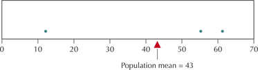
Note that the mean of the sample means $μ_{\bar{x}}$ equals the population mean $μ = 43$ . This is always true. So, we generalize it as follows.

Fact 1: Mean of the Sampling Distribution of $\bar{x}$

The mean of the sampling distribution of the sample mean $\bar{x}$ is the value of the population mean $μ$ . It can be denoted as $μ_{\bar{x}} = μ$ and read as “the mean of the sampling distribution of $\bar{x}$ is $μ$ .”

Note: It is convenient to number a set of important facts as we build toward the Central Limit Theorem for Means and the Central Limit Theorem for Proportions.

Now, the populations and samples you will encounter, both here and in the real world, are too large to list out all the possible sample means, as we did in Table 1. Instead, we will examine population distributions of data, with a mean $μ$ and standard deviation $σ$ , just as we did in Chapter 6. However, in Chapter 7, the population may or may not be normally distributed.

Next let's explore some more behavior of the sampling distribution of $\bar{x}$ , using a graphical example. In Example 1 we compare the population distribution of $X$ with the sampling distribution of $\bar{x}$ .

EXAMPLE 1 Sampling distribution of $\bar{x}$ for a normal population

In Example 37 in Chapter 6 (page 369), we saw that $X = temperature in Georgia$ in the month of April was normally distributed with a mean of $μ = 61.5 ° F$ and a standard deviation of $σ = 8 ° F$ . We want to compare this population distribution of $X$ with the sampling distribution of $\bar{x}$ . Using Minitab, 1000 samples of size $n = 4$ were generated from this normal distribution, and the sample means $\bar{x}$ were calculated for each sample. The histogram of green rectangles in Figure 2 was constructed, representing the sampling distribution of $\bar{x}$ for $n = 4$ .

Identify the shape of the sampling distribution of $\bar{x}$ .
Find the mean of the sampling distribution of $\bar{x}$ .
Use the Empirical Rule to estimate the standard deviation of the sampling distribution of $\bar{x}$ .
Compare the population distribution of $X$ with the sampling distribution of $\bar{x}$ .

Solution

Figure 2 shows the histogram (rectangles) of the means from the 1000 samples of size $n = 4$ .

As you may have expected, the histogram of rectangles representing the sampling distribution of $\bar{x}$ is normal.
The balance point of the sampling distribution is located at 61.5. Thus, the mean $μ_{\bar{x}}$ of the sampling distribution of $\bar{x}$ equals the population mean $μ = 61.5$ .
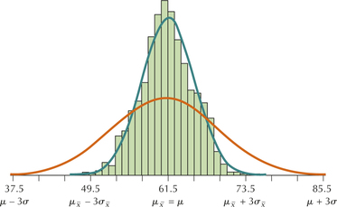
Figure 2 shows that almost all the sample means lie between 49.5 and 73.5. Recall that the Empirical Rule states that almost all the data from a normal distribution lie within 3 standard deviations of the mean. Thus, the distance $61.5 - 49.5 = 12$ represents 3 standard deviations. Thus, we estimate that the standard deviation of the sampling distribution of $\bar{x}$ is: $σ_{\bar{x}} = 12 / 3 = 4$ .
Page 398
Note the orange curve in Figure 2. This represents the distribution of the original normal temperature data, with $μ = 61.5$ and $σ = 8$ . Compare this to the green curve, which represents the sampling distribution of $\bar{x}$ , with mean $μ_{\bar{x}} = 61.5$ and $σ_{\bar{x}} = 4$ . Note that the spread (variability) of the sampling distribution is less than the spread of the original distribution of $X$ .

FIGURE 2 The sampling distribution of $\bar{x}$ (in green) has less spread (variability) than the original distribution $X$ (in orange).

In Example 1, we estimated the standard deviation of the sampling distribution of $\bar{x}$ to be $σ_{\bar{x}} = 4$ , compared with the original standard deviation $σ = 8$ . Fact 2 shows the relationship between these two quantities in general.

Note: Fact 2 is derived using methods found in texts on advanced statistics.

Fact 2: Standard Deviation of the Sampling Distribution of $\bar{x}$

The standard deviation of the sampling distribution of the sample mean $\bar{x}$ is

$σ_{\bar{x}} = σ / \sqrt{n}$

where $σ$ is the population standard deviation and $n$ is the sample size. $σ_{\bar{x}}$ is called the standard error of the mean.

Thus, for Example 1, $σ_{\bar{x}} = σ / \sqrt{n} = 8 / \sqrt{4} = 8 / 2 = 4$ , so our estimate was correct. Note the $\sqrt{n}$ in the denominator of the formula. Because of this factor, the larger the sample size, the tighter the resulting sampling distribution. Larger sample sizes lead to smaller variability, which results in more precise estimation.

EXAMPLE 2 Finding the mean and standard deviation of the sampling distribution of $\bar{x}$

According to the American Time Use Survey, the mean amount of sleep that 20- to 24-year-old women get per night is 9.3 hours (Source: Bureau of Labor Statistics¹). Assume that the population standard deviation is $σ = 1$ hour. Find the mean and standard deviation for the sampling distribution of $\bar{x}$ for the following sample sizes: (a) 4, (b) 100, (c) 400.

Solution

We have $μ_{\bar{x}} = μ = 9.3$ . Note that this value for $μ_{\bar{x}}$ does not depend on the sample size, so the value is true for any sample size. We also have $σ = 1$ .

$n = 4$ . Then, $σ_{\bar{x}} = \frac{σ}{\sqrt{n}} = \frac{1}{\sqrt{4}} = 0.5.$ The standard error of the mean for $n = 4$ is $σ_{\bar{x}} = 0.5 hours$ .
$n = 100$ . Then, standard error $σ_{\bar{x}} = \frac{σ}{\sqrt{n}} = \frac{1}{\sqrt{100}} = 0.1.$
$n = 400$ . Then, standard error $σ_{\bar{x}} = \frac{σ}{\sqrt{n}} = \frac{1}{\sqrt{400}} = 0.05.$

NOW YOU CAN DO

Exercises 9–16.

Page 399

YOUR TURN#1

For the situation in Example 2, find the mean and standard deviation for the sampling distribution of $\bar{x}$ for $n = 900$ .

(The solution is shown in Appendix A.)

What Does This Number Mean?

Consider $σ_{\bar{x}} = 0.1$ for $n = 100$ in Example 2(b). This is a measure of the variability of the sampling distribution of $\bar{x}$ for this sample size. That is, if we take samples of size 100, our estimation of the population mean amount of sleep $μ$ of all 20- to 24-year-old women will be within 0.1 hour (6 minutes) of the true population mean most of the time.

Recall in Example 1 that when the original population distribution is normal, the sampling distribution of $\bar{x}$ is also normal. This is true in general, as stated in Fact 3, which also includes what we have learned so far in Fact 1 and Fact 2.

Fact 3: Sampling Distribution of the Sample Mean for a Normal Population

When random samples of size $n$ are taken from a data distribution $X$ that is normally distributed, the sampling distribution of $\bar{x}$ is also normally distributed.
Thus, when random samples of size n are taken from a normal population with mean $μ$ and standard deviation $σ$ , the sampling distribution of the sample mean $\bar{x}$ is distributed as normal with mean $μ_{\bar{x}} = μ$ and standard error $σ_{\bar{x}} = σ / \sqrt{n}$ .
In other words, the sampling distribution of $\bar{x}$ is distributed as normal $(μ, σ / \sqrt{n})$ .

Note: Let the notation

$normal (μ, σ / \sqrt{n})$

denote a normal distribution with mean of $μ$ and standard deviation of $σ / \sqrt{n}$ .

The good news is that, once we know that the sampling distribution is normal, we can use the methods we learned in Section 6.5 to solve probability problems. Specifically, we can standardize and produce $Z$ , just as we would for any normal random variable, using Fact 4.

Fact 4: Standardizing a Normal Sampling Distribution for Means

When the sampling distribution of $\bar{x}$ is normal, we may standardize to produce the standard normal random variable $Z$ as follows:

$Z = \frac{\bar{x} - μ_{\bar{x}}}{σ_{\bar{x}}} = \frac{\bar{x} - μ}{σ / \sqrt{n}}$

where $μ$ is the population mean, $σ$ is the population standard deviation, and $n$ is the sample size.

2 Central Limit Theorem for Means

The discussion so far has been for the case when the original population is normally distributed. However, what if the population (distribution of $X$ ) is not normal? In this section, we use a simulation study to learn how the sampling distribution of the sample mean $\bar{x}$ for non-normal populations becomes approximately normal as the sample size increases.

EXAMPLE 3 Simulation study: sample means from a strongly skewed population

nutrition

The data set Nutrition contains nutrition information on a population of 961 foods.

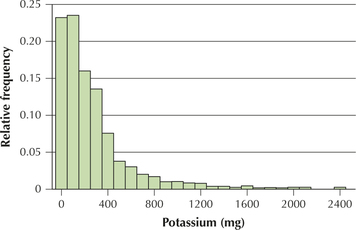
Construct a histogram of the potassium content of these 961 foods, and describe the shape of the population distribution.
Using Minitab, take 500 random samples of sizes $n = 10, 20, and 30$ from the population. Assess the normality of the resulting sampling distributions of $\bar{x}$ using histograms and normal probability plots.

Solution

A histogram of the potassium content of these foods is shown in Figure 3, revealing a strongly right-skewed, non-normal data set.
Page 400

FIGURE 3 Potassium content is strongly right-skewed, not normal.
Using Minitab, we take 500 random samples of size $n = 10$ from the population. The histograms of each set of 500 means are shown in Figure 4.
- $n = 10$ : The sampling distribution $\bar{x}$ is skewed (Figure 4a).
- $n = 20$ : The sampling distribution of $\bar{x}$ is still somewhat skewed (Figure 4b).
- $n = 30$ : Despite a few outliers, the sampling distribution of $\bar{x}$ is approximately normal (Figure 4c).
  
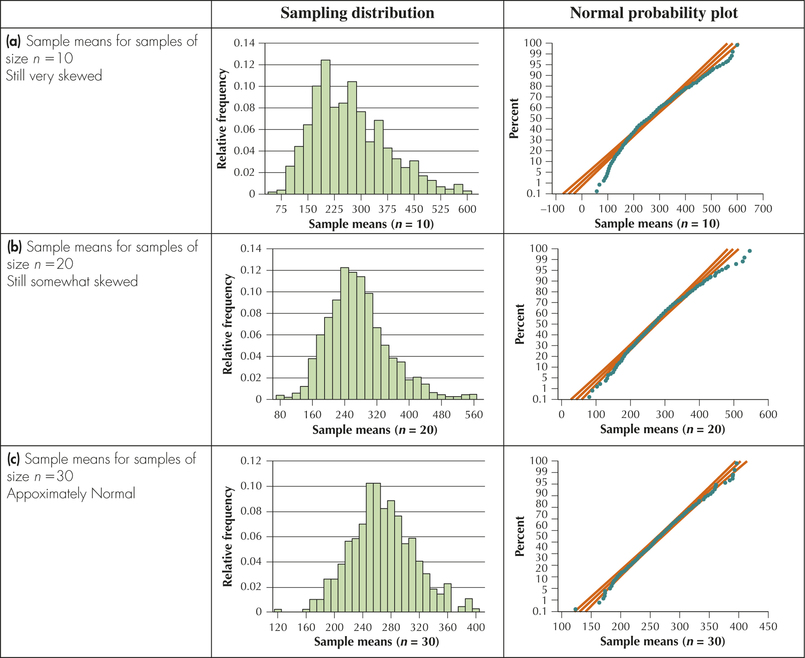  FIGURE 4 Sampling distribution of $\bar{x}$ and normal probability plots for $n = 10, 20, and 30$ .

The Central Limit Theorem applet allows you to experiment with various sample sizes and see how the Central Limit Theorem for Means behaves in action.

Page 401

For a skewed population, we have seen that the sampling distribution of the sample mean becomes approximately normal as the sample size reaches 30. For a less skewed population, we can expect that the sampling distribution of $\bar{x}$ approximates a normal distribution for smaller sample sizes. Our simulation study has shown us that regardless of the population, the sampling distribution of the sample mean becomes approximately normal as the sample size gets larger. We can then combine this statement with Fact 3 (page 399) to form the Central Limit Theorem for Means.

Central Limit Theorem for Means

When random samples of size $n$ are taken from a population with mean $μ$ and standard deviation $σ$ , the sampling distribution of the sample mean $\bar{x}$ becomes approximately normal $(μ, σ / \sqrt{n})$ as the sample size gets larger, regardless of the shape of the population.

How large does the sample size have to be before the Central Limit Theorem for Means takes effect? In general, it depends on the degree of symmetry, or skewness, of the population. In the simulation study (Figure 4), we saw that the sampling distribution of $\bar{x}$ was approximately normal, even for a skewed population when $n = 30$ . Thus, we shall abide by the following rule of thumb.

Rule of Thumb for When to Use the Central Limit Theorem for Means

We consider $n \geq 30$ as large enough to apply the Central Limit Theorem for Means for any population.

Developing Your Statistical Sense

The Central Limit Theorem

The Central Limit Theorem (CLT) is one of the most important results in statistics. Worldwide, much statistical inference is based on the CLT. It actually makes fairly intuitive sense, doesn't it? If we find the mean of a sample of data values, in many cases the extreme values will tend to balance out. However, remember that the mean is very sensitive to outliers. In a small sample, there may not be enough nonextreme values to balance the influence of the outliers. This is what was happening early in the potassium simulation (for example, Figure 4a). However, as the sample sizes increase, the influence of extreme values diminishes and the resulting sample means start to migrate toward the center.

Combining Fact 3 and the Central Limit Theorem for Means, we can identify three possible cases for the sampling distribution of $\bar{x}$ .

Three Possible Cases for the Sampling Distribution of the Sample Mean $\bar{x}$

Case 1. The population is normal. Therefore, the sampling distribution of $\bar{x}$ is normal (Fact 3, page 399).
Case 2. The population is either non-normal or of unknown distribution and the sample size is at least 30. Therefore, the sampling distribution of $\bar{x}$ is approximately normal (Central Limit Theorem for Means).
Case 3. The population is either non-normal or of unknown distribution and the sample size is less than 30. Therefore, we have insufficient information to conclude that the sampling distribution of the sample mean $\bar{x}$ is either normal or approximately normal.

Of course, in the real world, no one will tell you which of the three cases applies. You need to investigate the assumptions of each of the cases to determine for yourself which one applies.

Page 402

EXAMPLE 4 Is the sampling distribution of $\bar{x}$ normal?

For each of (a)–(c), determine whether the sampling distribution of $\bar{x}$ is normal, approximately normal, or unknown.

Assume SAT Math scores are normally distributed. Samples of size $n = 9$ are taken.
Assume SAT Math scores are not normally distributed. Samples of size $n = 36$ are taken.
Assume SAT Math scores are not normally distributed. Samples of size $n = 9$ are taken.

Solution

Here, the distribution of $X$ (SAT Math scores) is normally distributed, so the sampling distribution of $\bar{x}$ is automatically normal (Fact 3, page 399), regardless of the sample size. This is Case 1 from the Three Cases above.
Here, $X$ is not normal, but the sample size $n = 36$ is considered large because it is greater than 30. Thus, the Central Limit Theorem applies, so that the sampling distribution of $\bar{x}$ is approximately normal. This is Case 2 from the Three Cases above.
Here, we have neither normality nor a large sample size. Therefore, we have insufficient information to conclude that the sampling distribution of the sample mean $\bar{x}$ is either normal or approximately normal. This is Case 3 from the Three Cases above.

NOW YOU CAN DO

Exercises 17–26

3 Finding Probabilities Using a Sampling Distribution

We know that the sampling distribution of the sample mean $\bar{x}$ is normal when the population is normally distributed, so we can use the techniques of Section 6.5 to answer questions about the means of samples taken from normal populations.

EXAMPLE 5 Finding probabilities for the sample mean: Comparing $P (X > 80)$ with $P (\bar{x} > 80)$

Suppose the number of “likes” for Facebook pages is normally distributed with mean 70 likes and standard deviation 10 likes.

Find the probability that a randomly chosen Facebook user likes more than 80 pages.
Suppose we take many samples of size $n = 25$ Facebook users. Describe the sampling distribution of the sample mean.
Find the probability that a sample of 25 Facebook users will have a mean number of page likes greater than 80.

Solution

This is a normal probability problem, which we learned how to do in Section 6.5

$\begin{array}{l} P (X > 80) & = & P (\frac{X - 70}{10} > \frac{80 - 70}{10}) \\ = & P (Z > 1) = 1 - 0.8413 = 0.1587 \end{array}$

Page 403

using Case 2 from Table 8 in Chapter 6 (page 355), which shows how to find area to the right of a Z-value. Therefore, a 15.87% probability exists that a randomly chosen student will like more than 80 Facebook pages (Figure 5a).

It is especially important when answering sampling distribution problems to draw graphs of the original distribution of $X$ and the sampling distribution of $\bar{x}$ . Always draw graphs when solving probability problems. They bring in the “artistic side” of your brain to help the “analytic side” solve the problem.
We are given $μ = 70$ and $σ = 10$ . So, by Fact 1, $μ_{\bar{x}} = μ = 70$ . And by Fact 2,

$σ_{\bar{x}} = \frac{σ}{\sqrt{n}} = \frac{10}{\sqrt{25}} = 2.$

Next, we are given that the population of Facebook likes is normal. Therefore, by Fact 3, the sampling distribution of $\bar{x}$ is distributed as normal (70, 2) (see Figure 5b). This represents Case 1 from the Three Cases above.

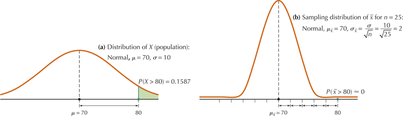FIGURE 5 Distribution of $X$ and sampling distribution of $\bar{x}$ for Example 5.
Once we know that the sample mean is normally distributed, we can standardize the sample mean number of page likes, as we have for other normal random variables. Just be sure to use $σ_{\bar{x}} = 2$ , the standard error of the mean, and not $σ = 10$ , the standard deviation for the population. $σ_{\bar{x}}$ is always smaller.

Applying Fact 4,

$Z = \frac{\bar{x} - μ_{\bar{x}}}{σ_{\bar{x}}} = \frac{\bar{x} - μ}{σ / \sqrt{n}} = \frac{\bar{x} - 70}{10 / \sqrt{25}} = \frac{\bar{x} - 70}{2}$

We need to standardize the value of 80 page likes, too.

$Z = \frac{80 - μ_{\bar{x}}}{σ_{\bar{x}}} = \frac{80 - μ}{σ / \sqrt{n}} = \frac{80 - 70}{10 / \sqrt{25}} = \frac{80 - 70}{2} = 5$

Thus,

$P (\bar{x} > 80) = P (\frac{\bar{x} - 70}{10 / \sqrt{25}} > \frac{80 - 70}{10 / \sqrt{25}}) = P (\frac{\bar{x} - 70}{2} > \frac{80 - 70}{2}) = P (Z > 5) \approx 0$

as shown in Figure 5b. Because $Z$ is standard normal, nearly all observations lie between −3 and 3. Thus, the $Z$ table does not go up to 5 because the probabilities are so close to 0. The TI-83 provides the more precise probability of $P (Z > 5) = 0.000000287$ , or about 3 in 10 million.

NOW YOU CAN DO

Exercises 27–32.

YOUR TURN#2

For the scenario in Example 5, find the probability that a sample of 25 Facebook users will have a mean number of page likes that is less than 75.

(The solution is shown in Appendix A.)

Page 404

What Does This Probability Mean?

There is essentially no chance that the sample mean number of page likes $\bar{x}$ will be greater than 80. Compare this to the nearly 16% chance that a particular Facebook user's number of page likes would be above 80. Figure 5 shows the graphs of the distributions of (a) the individual Facebook users, and (b) the means of sets of 25 users. Both distributions are centered at $μ_{\bar{x}} = μ = 70$ , but the standard deviations differ. The arrow in Figure 5a represents the standard deviation of $X, σ = 10$ , and it shows that $x = 80$ is only 1 standard deviation above the mean $μ = 70$ . The arrows in Figure 5b represent the standard error of the mean, $σ_{\bar{x}} = 2$ , and they illustrate that $\bar{x} = 80$ lies 5 standard errors above the mean $μ_{\bar{x}} = 70$ . Thus, group means are less variable than individual data values.

In Chapter 6, we found the percentiles of normally distributed random variables. The sampling distribution of $\bar{x}$ is normal, so we are able to find the percentiles of the $\bar{x}$ 's, too. Once the appropriate $Z$ -value is found, we use the following equation to transform the $Z$ -value into an $\bar{x}$ -value:

$\bar{x} = Z \cdot σ_{\bar{x}} + μ_{\bar{x}} = Z \cdot \frac{σ}{\sqrt{n}} + μ$

EXAMPLE 6 Finding a value of $\bar{x}$ , given a probability or area

Use the information in Example 5 to do the following:

Find the 95th percentile of the sample mean number of Facebook page likes from samples of size $n = 25$ .
Find the 5th percentile of the sample means.
What two symmetric values for the sample mean contain the middle 90% of all sample means between them?
Verify that $P (66.71 \leq \bar{x} \leq 73.29) = 0.90$ .

Solution

The 95th percentile of the sample mean number of Facebook likes is the value of $\bar{x}$ with area 0.95 to the left of it.

We want the 95th percentile, so we seek 0.95 on the inside of the $Z$ table. Because 0.95 is not in the $Z$ table, we take the closest value. The two closest values, 0.9495 and 0.9505, are equally close, so we split the difference. Working backward from 0.9495, we find $Z = 1.64$ , and for 0.9505 we find $Z = 1.65$ . Splitting the difference, we get $Z = 1.645$ . This value of $Z = 1.645$ is the 95th percentile of the standard normal distribution.

Because we are looking for a sample mean number of page likes, 1.645 is probably not the answer. We need to “unstandardize” by transforming this value of $Z$ to an $\bar{x}$ -value:

$\bar{x} = Z \cdot σ_{\bar{x}} + μ = 1.645 (2) + 70 = 73.29$

Thus, the 95th percentile of the sample means for the number of Facebook page likes is 73.29.
The sampling distribution is normal, so it is also symmetric. Thus, the 95th percentile and the 5th percentile are the same distance away from the mean. Because the 95th percentile is $(73.29 - 70) = 3.29$ above the mean, the 5th percentile must be 3.29 below the mean, or $(70 - 3.29) = 66.71$ .
This is just another way of asking for the 5th and 95th percentiles, which we found in parts (a) and (b). (See Figure 6.) The answer is 66.71 and 73.29.

Page 405

FIGURE 6 Middle 90% of the sample means.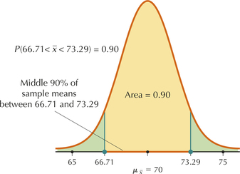
We seek $P (66.71 < \bar{x} < 73.29)$ , as shown in Figure 6. Proceeding with the calculations, we have, as expected,

$\begin{array}{l} P (66.71 < \bar{x} < 73.29) & = & P (\frac{66.71 - 70}{2} < \frac{\bar{x} - 70}{2} < \frac{73.29 - 70}{2}) \\ = & P (- 1.6454 < Z < 1.645) = 0.95 - 0.05 = 0.90 \end{array}$

NOW YOU CAN DO

Exercises 33–58.

YOUR TURN#3

Using the information in Example 5, find the 2.5th percentile of the mean number of Facebook page likes.

(The solution is shown in Appendix A.)

EXAMPLE 7 Finding probabilities using the Central Limit Theorem for Means

fuelefficiency

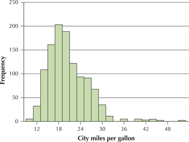
The data set FuelEfficiency contains information about the fuel efficiency of more than one thousand 2014 model year vehicles (Source: fueleconomy.gov). Figure 7 shows a histogram of the city miles per gallon (city mpg) of these vehicles, illustrating that the distribution is not normal, but somewhat right-skewed. The mean city mpg for all vehicles is $μ = 20$ , and the standard deviation is $σ = 6$ . Find the probability that a random sample of size $n = 36$ vehicles will have a mean city mpg greater than 21.

FIGURE 7 Population is skewed, so a large sample is needed to apply the Central Limit Theorem.

Solution

Clearly, the population is not normal, but the sample size $n = 36$ is large enough, so the Central Limit Theorem applies. The sampling distribution of the sample mean $\bar{x}$ is approximately normal. This is Case 2 from the Three Cases (page 401). Next, we need to find $μ_{\bar{x}}$ and $σ_{\bar{x}}$ . Facts 1 and 2 tell us that

Page 406

$μ_{\bar{x}} = μ = 20 and σ_{\bar{x}} = \frac{σ}{\sqrt{n}} = \frac{6}{\sqrt{36}} = 1$

Therefore, as the CLT indicates, the sampling distribution of $\bar{x}$ is approximately normal $(μ_{\bar{x}} = 20, σ_{\bar{x}} = 1)$ . We are then left to solve a normal probability problem using the methods of Section 6.5. Figure 8 shows the sampling distribution of $\bar{x}$ and the probability we are interested in, $P (\bar{x} > 21)$ . Using Fact 4, we standardize:

$Z = \frac{21 - μ_{\bar{x}}}{σ_{\bar{x}}} = \frac{21 - 20}{1} = 1$

Thus, $P (\bar{x} > 21) = P (Z > 1)$ , as shown in Figure 9. We therefore look up $Z = 1$ in the $Z$ table and subtract this table area (0.8413) from 1 to get the desired tail area:

$P (Z > 1) = 1 - 0.8413 = 0.1587$

The probability is 0.1587 that a random sample of 36 vehicles will have a mean city mpg greater than 21.

NOW YOU CAN DO

Exercises 59–70

FIGURE 8 Area to the right of

$\bar{x} = 21$ equals …
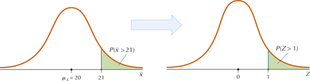
FIGURE 9 Area to the right of

$Z = 1$ .

YOUR TURN#4

For the situation in Example 7, find the probability that a random sample of size $n = 36$ vehicles will have a mean city mpg that is less than 18.5.

(The solution is shown in Appendix A.)

EXAMPLE 8 Finding two symmetric sample mean values using the Central Limit Theorem for Means

FIGURE 10

Refer to Example 7. If we take samples of size $n = 36$ , find the two symmetric values of $\bar{x}$ that contain the middle 95% of sample mean city mpg values.

Solution

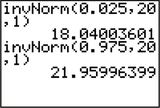
Here, we use the instructions from the Finding Percentiles for Any Normal Distribution portion of the Section 6.5 Step-by-Step Technology Guide on page 380. We have $μ_{\bar{x}} = 20$ and $σ_{\bar{x}} = 1$ . We want the middle 95% of sample means, so we ask the TI-83/84 calculator to give us the sample mean with 2.5% to the left of it and the sample mean with 97.5% to the left of it, as shown in Figure 10. We get ${\bar{x}}_{1} \approx 18.04$ as the 2.5th percentile of sample means and ${\bar{x}}_{2} \approx 21.96$ as the 97.5th percentile of sample means. These are the two symmetric values of the sample mean that contain the middle 95% of all sample mean city mpg values.

NOW YOU CAN DO

Exercises 71–80.

Page 407

YOUR TURN#5

For the situation in Example 7, if we take samples of size $n = 36$ , find the two symmetric values of $\bar{x}$ that contain the middle 90% of sample mean city mpg values.

(The solution is shown in Appendix A.)

EXAMPLE 9 Sometimes there is insufficient information to solve the problem

Using the same data set as in Example 8, suppose the sample size is only $n = 10$ . Now try again to find the probability that a random sample of size $n = 10$ vehicles will have a mean city mpg greater than 21.

Solution

The population is skewed (not normal) and the sample size $n = 10$ is less than the minimum $n = 30$ required to apply the Central Limit Theorem. Therefore, we have insufficient information to conclude that the sampling distribution of the sample mean $\bar{x}$ is either normal or approximately normal. This is Case 3 from the Three Cases (page 401). Unfortunately, we cannot find the probability that a random sample of $n = 10$ vehicles will have a mean city mpg greater than 21.

Trial of the Pyx: How Much Gold Is in Your Gold Coins?

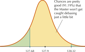
Medieval English kings devised a procedure to ensure that the coins of the realm contained the proper amount of gold. A sample of 100 of the gold coins that were cast each year was placed in a ceremonial box called the Pyx. At the chosen time, the Company of Goldsmiths jury weighed the gold coins. The mean weight of the coins was supposed to be 128 grams. If the mean weight was much less than 128 grams, the jury concluded that the Master of the Mint was cheating the crown by pocketing the excess gold, and he was severely punished. If the mean weight of the coins was within 0.32 gram of the expected 128 grams, the jury accepted the year's gold as pure. Thus, the mean weight had to lie between 127.68 grams and 128.32 grams.

Problem 1. Can we estimate what the jury used for a standard deviation?

Solution to Problem 1. Let's assume that “much less than” indicated a measurement that is 2 or more standard deviations below average. For the sampling distribution of $\bar{x}$ , then, this would indicate a range of $0.32 = 2 σ_{\bar{x}}$ between 127.68 and the mean 128. Therefore, $σ_{\bar{x}} = 0.16$ . And therefore, by the Empirical Rule, for instance, approximately 95% of the sample mean observations for the Trial of the Pyx would have been between 127.68 and 128.32. Because $σ_{\bar{x}} = σ / \sqrt{n}$ , it follows that $σ = \sqrt{100} \cdot 0.16 = 1.6 grams$ .

Problem 2. What were the chances that the Master of the Mint would have been caught and punished if he were in fact cheating the throne?

Solution to Problem 2. What if the Master of the Mint set the mean amount of gold per coin in the population of all coins to be $μ = 127.9 grams$ instead of the required 128, shortchanging the crown by a tenth of a gram of gold per coin? The jury would never have noticed this, would they?

Let's calculate the probability that the Master of the Mint would have passed the Trial of the Pyx if the mean amount of gold per coin had been only 127.9 grams. We've seen that the Master of the Mint would have passed the Trial of the Pyx if $127.68 < \bar{x} < 128.32$ . Now, because 100 is a large sample size, the Central Limit Theorem tells us that the sampling distribution of $\bar{x}$ is approximately normal, with

$μ_{\bar{x}} = μ = 127.9 and σ_{\bar{x}} = \frac{σ}{\sqrt{n}} = \frac{1.6}{\sqrt{100}} = 0.16$

Page 408

Standardizing using Fact 5:

$\begin{array}{l} Z & = & \frac{127.68 - μ_{\bar{x}}}{σ_{\bar{x}}} & = & \frac{127.68 - 127.9}{0.16} & \approx & - 1.38 & and \\ Z & = & \frac{128.32 - μ_{\bar{x}}}{σ_{\bar{x}}} & = & \frac{127.32 - 127.9}{0.16} & \approx & 2.63 \end{array}$

Solving using Table 8 in Chapter 6 (page 355):

$P (- 1.38 < Z < 2.63) = 0.9957 - 0.0838 = 0.9119$

That is, the chances of the crown accepting the coins as pure, even if the Master of the Mint had been shortchanging by a tenth of a gram per coin, were over 91% (Figure 11).

FIGURE 11 Sampling distribution if population mean gold weight is reduced to 127.9 grams.

Note: Sir William Sharington, 1493–1553, Master of the Mint during the turbulent Tudor era in England. He debased the currency, issued worthless coinage, and diverted the real gold to fund Thomas Seymour's conspiracy to topple the government and seize young King Edward VI. Sharington was arrested in 1548 or 1549, but he later received pardon and became Sheriff of Wiltshire for a short time before he died.

Problem 3. Would the Master of the Mint have been satisfied with this small amount of debasement? Would he have quit while he was ahead?

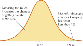
Solution to Problem 3. No way! The following year, the Master of the Mint decided to debase the currency even further, setting the mean amount of gold in the coins to be $μ = 127.3 grams per coin$ .

We need to find the probability of the Master passing the Trial of the Pyx if the mean amount of gold in a coin was 127.3 grams instead of the required 128 grams per coin. We use the same calculations, with $μ_{\bar{x}} = 127.3 grams$ . Standardizing:

$\begin{array}{l} Z & = & \frac{127.68 - μ_{\bar{x}}}{σ_{\bar{x}}} & = & \frac{127.68 - 127.3}{0.16} & \approx & 2.38 & and \\ Z & = & \frac{128.32 - μ_{\bar{x}}}{σ_{\bar{x}}} & = & \frac{128.32 - 127.3}{0.16} & \approx & 6.38 \end{array}$

Then, $P (2.38 < Z < 6.38) \approx 1 - 0.9913 = 0.0087$ .

In other words, the Master of the Mint actually would have stood very little chance—less than 1% probability—of passing the Trial of the Pyx if he cheated by this much (Figure 12).

England is a great country for retaining fine old traditions. Today, England's Company of Goldsmiths still operates the London Assay Office where the purity of the kingdom's coin is tested at the annual Trial of the Pyx.

Page 409

FIGURE 12 Sampling distribution if population mean gold weight is reduced to 127.3 grams.