9.7 Probability of a Type II Error and the Power of a Hypothesis Test
 This page includes Video Technology Manuals
OBJECTIVES By the end of this section, I will be able to …
- Calculate the probability of a Type II error for a Z test for μ.
- Compute the power of a Z test for μ and construct a power curve.
1 Probability of a Type II error
In Section 9.1, we defined a Type II error as follows:
Type II error: not rejecting H0 when H0 is false
For example, the criminal trial scenario on page 494 had the following hypotheses:
H0:defendant is not guiltyversusH0:defendant is guilty
In this case, a Type II error was to find the defendant not guilty (not reject H0) when in reality he did commit the crime (H0 is false). In this section, we learn how to calculate the probability of making a Type II error for a Z test for μ, called β (beta), and to use the value of β to compute the power of a Z test for μ.
Calculating β, the Probability of a Type II Error
Use the following steps to calculate β, the probability of a Type II error.
Step 1 Recall that Zcrit divides the critical region from the noncritical region. Let ˉxcrit be the value of the sample mean ˉx associated with Zcrit. The following table shows how to calculate ˉxcrit for the three forms of the hypothesis test.
Form of test Value of ˉxcrit Right-tailed H0:μ=μ0 vs. Ha:μ>μ0 ˉxcrit=μ0+Zcrit·σ√n Left-tailed H0:μ=μ0 vs. Ha:μ<μ0 ˉxcrit=μ0-Zcrit·σ√n Two-tailed H0:μ=μ0vs.Ha:μ≠μ0 ˉxcrit, lower=μ0-Zcrit·σ√n ˉxcrit, upper=μ0+Zcrit·σ√n Here, μ0 is the hypothesized value of the population mean, σ is the population standard deviation, and n is the sample size.
- Step 2 Let μa represent a particular value for the population mean μ chosen from the values indicated in the alternative hypothesis Ha. Draw a normal curve centered at μa, with the value or values of ˉxcrit from Step 1 indicated (see Example 34).
Step 3 Calculate β for the particular μa chosen using the following table.
| Form of test | β = probability of Type II error | |
|---|---|---|
| Right-tailed | H0:μ=μ0vs.Ha:μ>μ0 | The area under the normal curve drawn in Step 2 to the left of ˉxcrit. |
| Left-tailed | H0:μ=μ0vs.Ha:μ<μ0 | The area under the normal curve drawn in Step 2 to the right of ˉxcrit. |
| Two-tailed | H0:μ=μ0vs.Ha:μ≠μ0 | The area under the normal curve drawn in Step 2 between ˉxcrit, lower and ˉxcrit, upper. |
Let us illustrate the steps for calculating β, the probability of a Type II error, using an example.
EXAMPLE 34 Calculating β, the probability of a Type II error
ATM network operator Star Systems of San Diego reported that active users of debit cards used them an average of 11 times per month. Suppose we are interested in testing whether people use debit cards on average more than 11 times per month, using level of significance α=0.01. The hypotheses are
H0:μ=11versusHa:μ>11
where μ represents the population mean debit card usage per month. Suppose we have n=36, ˉx=11.5, and σ=3, and from Table 4 (page 500) we have Zcrit=2.33.
- State what a Type II error would be in this case.
- Let μa=13. That is, suppose the population mean debit card usage is actually 13 times per month. Calculate β, the probability of making a Type II error when μa=13.
Solution
- We make a Type II error when we do not reject H0 when H0 is false. In this case, a Type II error would be to conclude that the population mean debit card usage was 11 times per month when in actuality it was more than 11 times per month.
- We follow the steps for calculating β.
Step 1 We have a right-tailed test, so that
ˉxcrit=μ0+zcrit·σ√n=11+2.33·3√36=12.165
Step 2 Figure 49 shows the normal curve centered at μa=13, with ˉxcrit=12.165 labeled.
FIGURE 49 β probability of Type II error.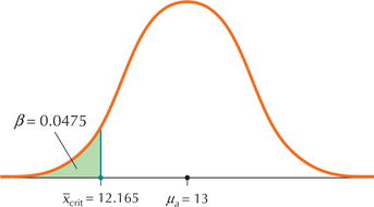
Step 3 The right-tailed test tells us that β equals the area under the normal curve drawn in Step 2 to the left of ˉxcrit=12.165. This is the shaded area in Figure 49. Area represents probability, so we have
β=p(ˉx<12.165)when μa=13
Standardizing with μa=13,σ=3, and n=36:
β=P(ˉx<12.165)=P(Z<12.165-133/√36)=P(Z<-1.67)=0.0475
Thus, β=0.0475. This represents the probability of making a Type II error, that is, of not rejecting the hypothesis that the population mean debit card usage is 11 times per month when in actuality it is 13 times per month.
NOW YOU CAN DO
Exercises 5–16.
2 Power of a Hypothesis Test
It is a correct decision to reject the null hypothesis when the null hypothesis is false. The probability of making this type of correct decision is called the power of the test.
Power of a Hypothesis Test
The power of a hypothesis test is the probability of rejecting the null hypothesis when the null hypothesis is false. Power is calculated as
power =1-β
EXAMPLE 35 Power of a hypothesis test
Calculate the power, for the particular alternative value of the mean, of the hypothesis test in Example 34.
Solution
The probability of a Type II error was found in Example 34 to be β=0.0475. Thus, the power of the hypothesis test is
power =1-β=1-0.0475=0.9525
The probability of correctly rejecting the null hypothesis is 0.9525.
NOW YOU CAN DO
Exercises 17–28.
 What if Scenario: Type II Errors and Power of the Test
Suppose that we have the same hypothesis test from Example 34 and the same value ˉxcrit=12.165. Now, what if we decrease μa such that it is less than 13 but still larger than 12.165? Describe what will happen to the following, and why:
- The probability of a Type II error, β
- The power of the test, 1-β
Solution
Consider Figure 50. The distribution of sample means remains centered at μa, so that a smaller μa will “slide” the normal curve toward the value of ˉxcrit=12.165. This results in a larger area to the left of 12.165, as you can see by comparing Figure 50 with Figure 49. Therefore, a smaller μa leads to an increase in the probability of a Type II error, β.
- As β increases, 1-β decreases. Therefore, a smaller μa leads to a decrease in the power of the test.
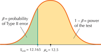 FIGURE 50 Smaller μa leads to an increase in β.
A power curve plots the values for the power of the test versus the values of μa.
EXAMPLE 36 Power curve
- Calculate the power of the hypothesis test from Example 34 for the following values of μa:11.0, 11.5, 12.0, 12.165, 12.5, 13.5.
- Construct the power curve by graphing the values for the power of the test on the vertical axis against the values of μa on the horizontal axis.
Solution
- We have ˉxcrit=12.165, σ=3,, and n=36. The calculations are provided in the following table.
μa Probability of Type II error: β Power of the test: 1-β 11.0 P(Z<12.165-113/√36)=P(Z<2.33)=0.9901 1-0.9901=0.0099 11.5 P(Z<12.165-11.53/√36)=P(Z<1.33)=0.9082 1-0.9082=0.0918 12.0 P(Z<12.165-123/√36)=P(Z<0.33)=0.6293 1-0.6293=0.3707 12.165 P(Z<12.165-12.1653/√36)=P(Z<0.00)=0.5 1-0.5=0.5 12.5 P(Z<12.165-12.53/√36)=P(Z<-0.67)=0.2514 1-0.2514=0.7486 13.5 P(Z<12.165-13.53/√36)=P(Z<-2.67)=0.0038 1-0.0038=0.9962 Figure 51 represents a power curve, because it plots the values for the power of the test on the vertical axis against the values of μa on the horizontal axis. Note that, as μa moves farther away from the hypothesized mean μ0=11, the power of the test increases. This is because it is more likely that the null hypothesis will be correctly rejected as the actual value of the mean μa gets farther away from the hypothesized value μ0.
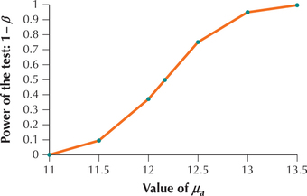 FIGURE 51 Power curve.
For completeness, we include the power for μa=13 from Example 35 in this power curve.
NOW YOU CAN DO
Exercises 29 and 30.