3.2 3.1 Scheduling Tasks
Assume that a certain number of identical processors (machines, humans, or robots) work on a series of tasks that make up a job. Associated with each task is a specified amount of time required to complete the task. For simplicity, we assume that any of the processors can work on any of the tasks. Our problem, known as the machine-scheduling problem, is to decide how the tasks should be scheduled so that the completion time for the tasks collectively is as early as possible.
Even with these simplifying assumptions, complications in scheduling arise. Some tasks may be more important than others and perhaps should be scheduled first. When “ties” occur, they must be resolved by special rules. As an example, suppose we are scheduling patients to be seen in a hospital emergency room staffed by one doctor. If two heavily bleeding patients arrive simultaneously, one with a bleeding thigh, the other with a bleeding arm, which patient should be treated first? Suppose the doctor treats the arm patient first, and while treatment is going on, a person in cardiac arrest or having a stroke arrives. Scheduling rules must establish appropriate priorities for cases such as these.
Another common complication arises with jobs consisting of several tasks that cannot be done in an arbitrary order. For example, if the job of putting up a new house is treated as a scheduling problem, the task of laying the foundation must precede the task of putting up the walls, which in turn must be completed before work on the roof can begin. The electrical system can be scheduled for installation later.

Assumptions and Goals
To simplify our analysis, we need to make clear and explicit assumptions:
- If a processor starts work on a task, the work on that task will continue without interruption until the task is completed.
- No processor stays voluntarily idle. In other words, if there is a processor free and a task available to be worked on, then that processor immediately begins work on that task.
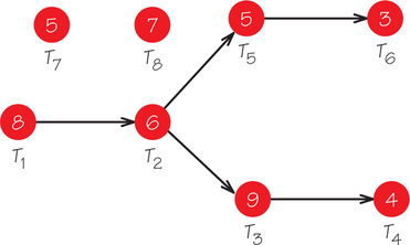
- The requirements for ordering the tasks are given by an order-requirement digraph. (A typical example is shown in Figure 3.1, with task times highlighted within each vertex. The ordering of the tasks imposed by the order-requirement digraph often represents constraints of physical reality. For example, you cannot fly a plane until it has taken fuel on board.)
- The tasks are arranged in a priority list that is independent of the order requirements. (The priority list is a ranking of the tasks according to some criterion of “importance.”)
EXAMPLE 1![]() Home Construction
Home Construction
Let’s see how these assumptions might work for an example involving a home construction project. In this case, the processors are human workers with identical skills. Assumption 1 means that once a worker begins a task, the work on this task is finished without interruption. Assumption 2 means that no worker stays idle if there is some task for which the predecessors are finished. Assumption 3 requires that the ordering of the tasks be summarized in an order-requirement digraph. This digraph would code facts such as that the site must be cleared before the task of laying the foundation is begun. Assumption 4 requires that the tasks be ranked in a list from some perspective, perhaps a subjective view.
The task with highest priority rank is listed first in the list, followed left to right by the other tasks in priority rank. The priority list might be based on the size of the payments made to the construction company when a task is completed, even though these payments have no relation to the way the tasks must be done, as indicated in the order-requirement digraph. Alternatively, the priority list might reflect an attempt to find an algorithm to schedule the tasks needed to complete the whole job more quickly.
When considering a scheduling problem, there are various goals we might want to achieve. Among them are the following:
- Goal 1. Minimizing the completion time of the tasks that make up the job.
- Goal 2. Minimizing the total time that processors are idle.
- Goal 3. Finding the minimum number of processors necessary to finish the job by a specified time.
In the context of the construction example, Goal 1 would complete the home as quickly as possible. Goal 2 would ensure that workers, who are perhaps paid by the hour, were not paid for doing nothing. One way of doing so would be to hire one fewer worker even if it means the house takes longer to finish. Goal 3 might be reasonable if the family wants the house done before the first day of school, even if they have to pay a lot more workers to get the house done by this time.
For now we will concentrate on Goal 1, finishing all the tasks that make up the job at the earliest possible time. Note, however, that optimizing for one goal may not optimize for another. Our discussion here goes beyond what was discussed in Chapter 2 (see Section 2.4) by dealing with how to assign tasks in a job to the processors that do the work. To build a new outpatient clinic involves designing a schedule for who will do what work when.
List-Processing Algorithm
The scheduling problem we have described sounds more complicated than the traveling salesman problem (TSP). Indeed, like the TSP, it is known to be NP-complete. This means that it is unlikely anyone will ever find a computationally fast algorithm that can find an optimal solution for scheduling problems involving a very large number of tasks. Thus, we will be content to seek a solution method that is computationally fast and gives only approximately optimal answers.
List-Processing Algorithm: Part I and Ready Task PROCEDURE
The algorithm we use to schedule tasks is the list-processing algorithm. In describing it, we will call a task ready at a particular time if all its predecessors as indicated in the order-requirement digraph have been completed at that time. In Figure 3.1 at time 0, the ready tasks are T1, T7, and T8, while T2 cannot be ready until 8 time units after T1 is started. The algorithm works as follows: At a given time, assign to the lowest-numbered free processor the first task on the priority list that is ready at that time and that hasn’t already been assigned to a processor.
In applying this algorithm, we will need to develop skill at coordinating the use of the information in the order-requirement digraph and the priority list. It will be helpful to cross out the tasks in the priority list as they are assigned to a processor to keep track of which tasks remain to be scheduled.
EXAMPLE 2![]() Applying the List-Processing Algorithm
Applying the List-Processing Algorithm
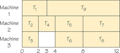
Let’s apply the list-processing algorithm to one possible priority list—T8, T7, T6, …, T1—using two processors and the order-requirement digraph in Figure 3.1. The result is the schedule shown in Figure 3.2, where idle processor time (time during which a processor is not at work on a task) is indicated by white. How does the list-processing algorithm generate this schedule?
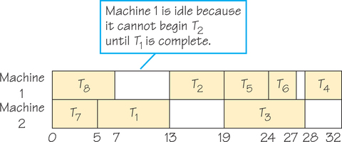
T8 (task 8) is first on the priority list and ready at time 0 since it has no predecessors. It is assigned to the lowest-numbered free processor, processor 1. Task 7, next on the priority list, is also ready at time 0 and thus is assigned to processor 2. The first processor to become free is processor 2 at time 5. Recall that by assumption 1, once a processor starts work on a task, its work cannot be interrupted until the task is complete. Task 6, the next unassigned task on the list, is not ready at time 5, as can be seen by consulting Figure 3.1. The reason task 6 is not ready at time 5 is that task 5 has not been completed by time 5. In fact, at time 5, the only ready task on the list is T1, so that task is assigned to processor 2. At time 7, processor 1 becomes free, but no task becomes ready until time 13.
Thus, processor 1 stays idle from time 7 to time 13. At this time, because T2 is the first ready task on the list not already scheduled, it is assigned to processor 1. Processor 2, however, stays idle because no other ready task is available at this time. The remainder of the scheduling shown in Figure 3.2 is completed in this manner.
We can summarize this procedure as follows:
List-Processing Algorithm: Part II PROCEDURE
As the priority list is scanned from left to right to assign a task to a processor at a particular time, we pass over tasks that are not ready to find tasks that are ready. If no task can be assigned in this manner, we keep one or more processors idle until such time that, reading the priority list from the left, there is a ready task not already assigned. After a task is assigned to a processor, we resume scanning the priority list for unassigned tasks, starting over at the far left.
When Is a Schedule Optimal?
The schedule in Figure 3.2 has a lot of idle time, so it may not be optimal. Indeed, if we apply the list-processing algorithm for two processors to another possible priority list T1, …, T8, using the digraph in Figure 3.1, the resulting schedule is that shown in Figure 3.3.
Here are the details of how we arrived at this schedule. Remember that we must coordinate the list T1, T2, …, T8 with the information in the order-requirement digraph shown in Figure 3.3a. At time 0, task T1 is ready, so this task is assigned to processor 1. However, at time 0, tasks T2, T3, …, T6 are not ready because their predecessors are not done. For example, T2 is not ready at time 0 because T1, which precedes it, is not done at time 0. The first ready task on the list, reading from left to right, that is not already assigned is T7, so task T7 gets assigned to processor 2. Both processors are now busy until time 5, at which point processor 2 becomes available to work on another task (Figure 3.3b).
Tasks T1 and T7 have been assigned. Reading from left to right along the list, the first task not already assigned whose predecessors are done by time 5 is T8, so this task is started at time 5 on processor 2; processor 2 will continue to work on this task until time 12, because the task time for this task is 7 time units. At time 8, processor 1 becomes free, and reading the list from left to right, we find that T2 is ready (because T1 has just been completed). Thus, T2 is assigned to processor 1, which will stay busy on this task until time 14. At time 12, processor 2 becomes free, but the tasks that have not already been assigned from the list (T3, T4, T5, T6) are not ready, because they depend on T2 being completed before these tasks can start. Thus, processor 2 must stay idle until time 14. At this time, T3 and T5 become ready. Since both processors 1 and 2 are idle at time 14, the lower numbered of the two, processor 1, gets to start on T3 because it is the first ready task remaining to be assigned on the list scanned from left to right. Task T5 gets assigned to processor 2 at time 14. The remaining tasks are assigned in a similar manner.
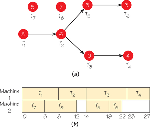
The schedule shown in Figure 3.3b is optimal because the path T1, T2, T3, T4, with length 27, is the critical path in the order-requirement digraph. As we saw in Chapter 2, the earliest completion time for the job made up of all the tasks is the length of the longest path in the order-requirement digraph. Different lists can give rise to the same or different optimal scheduling diagrams. The optimal schedule may have a completion time equal to or longer than the length of the critical path, but it cannot have a completion time shorter than the length of the critical path.
There is another way of relating optimal completion time to the completion time that is yielded by the list-processing algorithm. Suppose we add all the task times given in the order-requirement digraph and divide by the number of processors. The completion time using the list-processing algorithm must be at least as large as this number. For example, the task times for the order-requirement digraph in Figure 3.3a sum to 47. Thus, if these tasks are scheduled on two processors, the completion time is at least 472=23.5 (in fact, 24, because the list-processing algorithm applied to integer task times must yield an integer solution), whereas for four processors the completion time is at least 474 (in fact, at least 12).
Why is it helpful to take the total time to do all the tasks in a job and divide this number by the number of processors? Think of each task that must be scheduled as a rectangle that is 1 unit high and t units wide, where t is the time allotted for the task. Think of the scheduling diagram with m processors as a rectangle that is m units high and whose width, W, is the completion time for the tasks. The scheduling diagram is to be filled up (packed) by the rectangles that represent the tasks. How small can W be? The area of the rectangle that represents the scheduling diagram must be at least as large as the sum of all the rectangles representing tasks that fit into it. The area of the scheduling diagram rectangle is mW. The combined areas of all the tasks, plus the area of rectangles corresponding to idle time, equal mW. Width W is smallest when the idle time is zero. Thus, W must be at least as big as the sum of all the task times divided by m.
Sometimes the estimate for completion time given by the list-processing algorithm from the length of the critical path gives a more useful value than the approach based on adding task times. Sometimes the opposite is true. For the order-requirement digraph in Figure 3.1, except for a schedule involving one processor, the critical-path estimate is superior. For some scheduling problems, both these estimates may be poor.
The number of priority lists that can be constructed if there are n tasks is n! and can be computed using the fundamental principle of counting. For example, for eight tasks, T1, …, T8, there are 8×7×6…×1=40,320 possible priority lists. For different choices of the priority list, the list-processing algorithm may schedule the tasks, subject to the constraints of the order-requirement digraph, in different ways. More specifically, two different lists may yield different completion times or the same completion time, but the order in which the tasks are carried out will be different. It is also possible that two different lists produce identical ordering of the assignments of the tasks to processors and completion times. Soon we will see a method that can be used to select a list that, if we are lucky, will give a schedule with a relatively good completion time. In fact, no method is known, except for very specialized cases, of how to choose a list that can be guaranteed to produce an optimal schedule when the list algorithm is applied to it. In a nutshell, designing good schedules is difficult.
Self Check 1
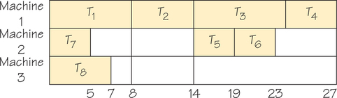
Apply the list-processing algorithms to the list with the tasks in numerical order for the order-requirement digraph in Figure 3.3 with three processors.
Strange Happenings
The list-processing algorithm involves four factors that affect the final schedule. The answer we get depends on the following:
- The times to carry out the tasks
- Number of processors
- Order-requirement digraph
- Ordering of the tasks on the priority list
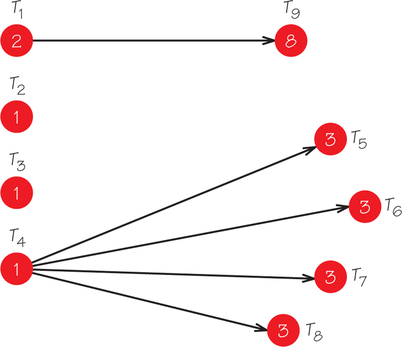
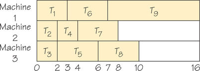
To see the interplay of these four factors, consider another scheduling problem, this time asociated with the order-requirement digraph shown in Figure 3.4. (The highlighted numbers are task time lengths.) The schedule generated by the list-processing algorithm applied to the list T1, T2, …, T9, using three processors, is given in Figure 3.5.
Treating the list T1, …, T9 as fixed, how might we make the completion time earlier? Our alternatives are to pursue one or more of these strategies:
- Reduce task times.
- Use more processors.
- “Loosen” the constraints by having fewer directed edges in the order-requirement digraph.

Let’s consider each alternative in turn, changing one feature of the original problem at a time, and see what happens to the resulting schedule. If we use strategy 1 and reduce the time of each task by one unit, we would expect the completion time to go down. Figure 3.6 shows the new order-requirement digraph, and Figure 3.7 shows the schedule produced for this problem, using the list-processing algorithm with three processors applied to the list T1, …, T9.
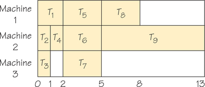
The completion time is now 13—longer than the completion time of 12 for the case (Figure 3.5) with longer task times. This is unexpected! Let’s explore further and see what happens.
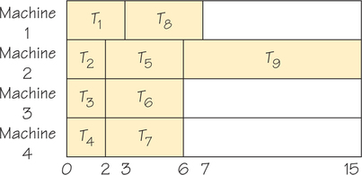
Next we consider strategy 2, increasing the number of machines. Surely, this should speed matters up. When we apply the list-processing algorithm to the original graph in Figure 3.4, using the list T1, …, T9 and four machines, we get the schedule shown in Figure 3.8. The completion time is now 15—an even later completion time than for the previous alteration.
Finally, we consider strategy 3, trying to shorten completion time by erasing all constraints (edges with arrows) in the order-requirement digraph shown in Figure 3.4. By increasing flexibility of the ordering of the tasks, we might guess we could finish our tasks more quickly. Figure 3.9 shows the schedule using the list T1, …, T9—now it takes 16 units! This is the worst of our three strategies to reduce completion time.
The failures we have encountered here are surprising at first glance, but they are typical of what can happen when a situation is too complex to analyze with naïve intuition. The value of using mathematics rather than intuition or trial and error to study scheduling and other problems is that it points out flaws that can occur in unguarded intuitive reasoning.
It is tempting to believe that we can make an adjustment in the rules for scheduling that we adopted to avoid the paradoxical behavior that has just been illustrated. Unfortunately, operations research experts have shown that there are no “simple fixes.” This means that, in practice, for large scheduling problems such as those that face our medical centers and transportation system, finding the best solution to a particular scheduling problem cannot be guaranteed (see Spotlight 3.1).