11.4 Oligopoly with Identical Goods: Cournot Competition
435
Model Assumptions Cournot Competition with Identical Goods
Firms sell identical products.
Firms compete by choosing a quantity to produce.
All goods sell for the same price—
the market price, which is determined by the sum of the quantities produced by all the firms in the market. Firms choose quantities simultaneously.
When firms sell identical goods, the Bertrand competition model results in the same equilibrium that we find in a perfectly competitive market, where price equals marginal cost. Because consumers care only about the price of the good (the product is identical across firms), each firm faces a demand that is perfectly elastic. Any increase in a firm’s price results in it losing all of its market share. The demand for the product will go to the firm offering the lowest price.
But what if firms face capacity constraints, and thus a limit on how much demand they can fill in the short run? With this restriction, if a firm undercuts another’s price, it can only steal as many customers as it has available capacity, and this capacity is probably not the size of the whole market.
In this model, there won’t be as much pressure for a firm to respond to price cuts because each firm will not lose all of its customers even if it keeps its price higher than that of a competitor. In fact, if the capacity of the low-
In this situation, the critical issue is for a firm to determine how much capacity it has and thus what quantity it can produce.
Setting Up the Cournot Model
Cournot competition
Oligopoly model in which each firm chooses its production quantity.
We raise the idea of capacity constraints to motivate another major oligopoly model, Cournot competition (named after its first modeler, Augustin Cournot—
In Cournot competition, firms produce identical goods and choose a quantity to produce rather than a price at which to sell the good. Individual firms do not control the price of their goods as they do in the Bertrand model. First, all firms in the industry decide how much they will produce; then based on the quantity produced by all firms, the market demand curve determines the price at which all firms’ output will sell. In Chapter 9, we learned that when dealing with a monopolist, the price-
To be more specific, let’s say there are two firms in a Cournot oligopoly, Firm 1 and Firm 2. (There can be more; we keep it at two to make it easy.) Each has a constant marginal cost of c, and both firms independently and simultaneously choose their production quantities q1 and q2. The good’s inverse demand curve is
P = a – bQ
where Q is the total quantity produced in the market: Q = q1 + q2.
436
Firm 1’s profit π1 is the quantity q1 it produces times the difference between the market price P and its production costs c, or
π1 = q1 × (P – c )
Substituting the inverse demand equation for P, we find that
π1 = q1 × [a – b (q1 + q2 ) – c ]
Similarly, Firm 2’s profits are given by the equation
π2 = q2 × [a – b ( q1 + q2 ) – c ]
These two profit equations make clear that the firms in this oligopoly strategically interact. Firm 1’s profit is not just a function of its own quantity choice q1, but also of its competitor’s quantity q2. Likewise, Firm 2’s profit is affected by Firm 1’s output choice. The logic is that each firm’s production choice, through its influence on the market price P, affects the other firm’s profit.
An example of an industry that is like the Cournot model is the crude oil industry. Crude oil is a commodity; consumers are indifferent about oil from different sources. The price of oil is set on a worldwide market, and it depends on the total amount of oil supplied at a given time. Therefore, it’s realistic to assume that oil producers, even those such as Saudi Arabia or Iran with large oil reserves, do not choose the price of their outputs. They just choose how much to produce. (As we discussed earlier, OPEC chooses production quantity targets, not prices.) Oil traders observe these production decisions for all oil producers, and they bid oil’s market price up or down depending on how the total quantity produced (the market supply) compares to current demand. This price-
Equilibrium in a Cournot Oligopoly
Finding the equilibrium for a Cournot oligopoly will be easier to follow using an example. Suppose for simplicity that only two countries pump oil, Saudi Arabia and Iran. Both have a marginal cost of production of $20 per barrel. Also assume that the inverse demand curve for oil is P = 200 – 3Q, where P is in dollars per barrel and Q is in millions of barrels per day.
Finding the equilibrium for the Cournot model is similar to doing so for a monopoly, but with the one change noted above: The market quantity Q is the sum of the quantities produced in Saudi Arabia qS and Iran qI , rather than just the monopolist’s output: Q = qS + qI . After recognizing this difference, we follow the same steps used to solve for a monopoly’s profit-
Let’s examine Saudi Arabia’s profit maximization first. As we learned in Section 9.2, we can more easily find a firm’s marginal revenue curve by starting with its inverse demand curve. Therefore, we start by writing the inverse demand curve equation in terms of the quantity choices of each country:
P = 200 – 3Q = 200 – 3(qS + qI) = 200 – 3qS – 3qI
Because the slope of the marginal revenue curve is twice the slope of the inverse demand function, Saudi Arabia’s marginal revenue curve is8
MRS = 200 – 6 qS – 3qI
437
Saudi Arabia maximizes profit when it produces the quantity at which its marginal revenue equals its marginal cost:
200 – 6qS – 3qI = 20
We can solve this equation for Saudi Arabia’s profit-
qS = 30 – 0.5qI
This outcome differs from the monopoly outcome: If Saudi Arabia were a monopoly, setting marginal revenue equal to marginal cost would result in a single quantity Q because its quantity supplied qS would be the market quantity supplied Q. In this example, however, Saudi Arabia’s profit-
qI = 30 – 0.5qS
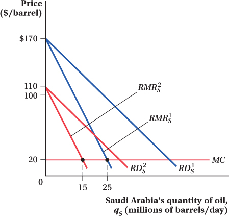
This result shows that one country’s output choice effectively decreases the demand for the other country’s output. That is, the demand curve for one country’s output is shifted in by the amount of the other country’s output. If the Saudis expect Iran to produce, say, 10 million barrels per day (bpd), then Saudi Arabia would effectively be facing the demand curve
P = 200 – 3qS – 3qI = 200 – 3qS – 3(10) = 170 – 3qS
If it expected Iran to pump out 20 million bpd, Saudi Arabia would face the demand curve
P = 200 – 3qS – 3(20) = 140 – 3qS
residual demand curve
In Cournot competition, the demand remaining for a firm’s output given competitor firms’ production quantities.
This demand that is left over to one country (or more generally, firm), taking the other country’s output choice as given, is called the residual demand curve. We just derived Saudi Arabia’s residual demand curves for two of Iran’s different production choices, 10 and 20 million bpd.
residual marginal revenue curve
A marginal revenue curve corresponding to a residual demand curve.
In effect, a firm in a Cournot oligopoly acts like a monopolist, but one that faces its residual demand curve rather than the market demand curve. The residual demand curve, like any regular demand curve, has a corresponding marginal revenue curve (it’s called . . . wait for it . . . the residual marginal revenue curve). The firm produces the quantity at which its residual marginal revenue equals its marginal cost. That’s why Saudi Arabia’s optimal quantity is the one that sets 200 – 6qS – 3qI = 20. The left-
How does the profit-
 and
and  As a result, Saudi Arabia’s optimum output decreases to 15 million bpd.
Each competitor’s profit-
438
To see what that implies for a Cournot oligopoly, note that the equation for each country’s profit-
reaction curve
A function that relates a firm’s best response to its competitor’s possible actions. In Cournot competition, this is the firm’s best production response to its competitor’s possible quantity choices.
Cournot Equilibrium: A Graphical Approach We can show this graphically in Figure 11.4. Saudi Arabia’s output is on the vertical axis and Iran’s output is on the horizontal axis. The curves illustrated are reaction curves. A reaction curve shows the best production response a country (or firm, in a more general oligopoly context) can make given the other country’s/firm’s action. Because both reaction curves are downward-
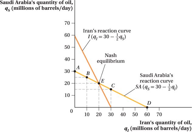
Reaction curve SA shows Saudi Arabia’s best response to any production choice of Iran—
Line I is the corresponding reaction curve for Iran’s profit-
439
Each country realizes that its actions affect the desired actions of its competitor, which in turn affect its own optimal action, and so on. This back-
Cournot Equilibrium: A Mathematical Approach In addition to finding the Cournot equilibrium graphically, we can solve for it algebraically by solving for the output levels that equate the two reaction curves. One way to do this is to substitute one equation into the other to get rid of one quantity variable and solve for the remaining one. For example, if we substitute Iran’s reaction curve into Saudi Arabia’s reaction curve for qI , we find
qS = 30 – 0.5qI = 30 – 0.5(30 – 0.5qS )
= 30 – 15 + 0.25qS
0.75qS = 15
qS = 20
Thus, the equilibrium output for Saudi Arabia is 20 million bpd. If we substitute this value back into Iran’s reaction curve, we find that qI = 30 – 0.5qS = 30 – 0.5(20) = 20. Iran’s optimal production is also 20 million bpd. Equilibrium point E in Figure 11.4 has the coordinates (20, 20), and total industry output is 40 million bpd.
440
The equilibrium price of oil at this point can be found by plugging these production decisions into the inverse market demand curve. Doing so gives P = 200 – 3(qS + qI ) = 200 – 3(20 + 20) = $80 per barrel. Each country’s profit is 20 million bpd × ($80 – $20) = $1,200 million = $1.2 billion per day, so the industry’s total profit is $2.4 billion per day.
 See the problem worked out using calculus
figure it out 11.2
For interactive, step-
OilPro and GreaseTech are the only two firms that provide oil changes in a local market in a Cournot duopoly (a two-
Determine each firm’s reaction curve and graph it.
How many oil changes will each firm produce in Cournot equilibrium?
What will the market price for an oil change be?
How much profit does each firm earn?
Solution:
Start by substituting Q = qO + qG into the market inverse demand curve:
P = 100 – 2Q = 100 – 2(qO + qG ) = 100 – 2qO – 2qG
From this inverse demand cure, we can derive each firm’s marginal revenue curve:
MRO = 100 – 4qO – 2qG
MRG = 100 – 2qO – 4qG
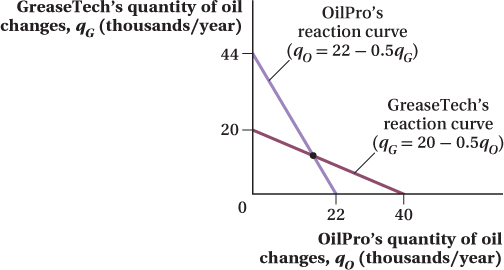
Each firm will set its marginal revenue equal to its marginal cost to maximize profit. From this, we can obtain each firm’s reaction curve:
MRO = 100 – 4qO – 2qG = 12
4qO = 88 – 2qG
qO = 22 – 0.5qG
MRG = 100 – 2qO – 4qG = 20
4qG = 80 – 2qO
qG = 20 – 0.5qO
These reaction curves are shown in the figure below.
To solve for equilibrium, we need to substitute one firm’s reaction curve into the reaction curve for the other firm:
qO = 22 – 0.5qG
qO = 22 – 0.5(20 – 0.5qO) = 22 – 10 + 0.25qO = 12 + 0.25qO
0.75qO = 12
qO = 16
qG = 20 – 0.5qO = 20 – 0.5(16) = 20 – 8 = 12
441
Therefore, OilPro produces 16,000 oil changes per year, while GreaseTech produces 12,000.
We can use the market inverse demand curve to determine the market price:
P = 100 – 2Q = 100 – 2(qO + qG ) = 100 – 2(16 + 12) = 100 – 56 = 44
The price will be $44 per oil change.
OilPro sells 16,000 oil changes at a price of $44 for a total revenue TR = 16,000 × $44 = $704,000. Total cost TC = 16,000 × $12 = $192,000. Therefore, profit for OilPro is π = $704,000 – $192,000 = $512,000.
GreaseTech sells 12,000 oil changes at a price of $44 for a total revenue of TR = 12,000 × $44 = $528,000. Total cost TC = 12,000 × $20 = $240,000. Thus, GreaseTech’s profit is π = $528,000 – $240,000 = $288,000.
Note that the firm with the lower marginal cost produces more output and earns a greater profit.
Comparing Cournot to Collusion and to Bertrand Oligopoly
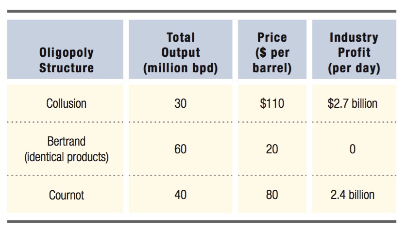
Let’s compare this equilibrium in a Cournot oligopoly (Q = 40 million bpd at P = $80) and profit ($2.4 billion per day) to the outcomes in other oligopoly models we’ve analyzed. These results are described in Table 11.2.
Collusion Let’s first suppose Saudi Arabia and Iran can actually get their acts together and collude to act like a monopolist. In that case, they would treat their separate production decisions qI and qS as a single total output Q = qS + qI . Following the normal marginal-
442
Bertrand Oligopoly with Identical Products Next, let’s consider the Nash equilibrium if the two countries competed as in the Bertrand model with identical products. In this case, we know that price will equal marginal cost, so P = $20. Total demand at this price is determined by plugging $20 into the demand curve: P = 20 = 200 – 3Q, or Q = 60 million bpd. The two countries would split this demand equally, with each selling 30 million bpd. Because both countries sell at a price equal to their marginal cost, each earns zero profit. At the Bertrand equilibrium, output quantity is higher than at the Cournot equilibrium, price is lower, and there is no profit.
Summary To summarize, then, in terms of total industry output, the lowest is the collusive monopoly outcome, followed by Cournot, then Bertrand:
Qm < Qc < Qb
The order is the opposite for prices, with Bertrand prices the lowest and the collusive price the highest:
Pb < Pc < Pm
Similarly, profit is lowest in the Bertrand case (at zero), highest under collusion, with Cournot in the middle:
πb = 0 < πc < πm
Therefore, the Cournot oligopoly outcome is something between those for monopoly and Bertrand oligopoly (for which the outcome is equivalent to perfect competition). And, unlike the collusive and Bertrand outcomes, the price and output in the Cournot equilibrium depend on the number of firms in the industry.
What Happens If There Are More Than Two Firms in a Cournot Oligopoly?
These intermediate outcomes are for a market with two firms. If there are more than two firms in a Cournot oligopoly, the total quantity, profits, and price remain between the monopoly and perfectly competitive extremes. However, the more firms there are, the closer these outcomes get to the perfectly competitive case, with price equaling marginal cost and economic profits being zero. Having more competitors means that any single firm’s supply decision becomes a smaller and smaller part of the total market. Its output choice therefore affects the market price less and less. With a very large number of firms in the market, a producer essentially becomes a price taker. It therefore behaves like a firm in a perfectly competitive industry, producing where the market price equals its marginal cost. Most Cournot markets are not at this limit, so price is usually above marginal cost, but for intermediate cases, more firms in a Cournot oligopoly lead to lower prices, higher total output, and lower average firm profits.
Cournot versus Bertrand: Extensions
The fact that the intensity of competition changes with the number of firms in the market is a nice feature of the Cournot model. This prediction is more in line with many people’s intuitive view of oligopoly than the Bertrand model’s prediction that anything more than a single firm leads to a perfectly competitive outcome. The downside of the Cournot framework is that it’s a bit more of a stretch than usual to assume that companies can only compete in their quantity choices and have no ability to charge different prices. How many oligopolies could that describe? Oil seems a very special case.
443
Economists David Kreps and José A. Scheinkman examined this assumption in more detail. They proved an important result (though it’s too mathematically advanced to detail here) that helps expand the applicability of the Cournot model.9 Kreps and Scheinkman showed that under certain conditions, even if firms actually set their prices instead of quantities, the industry equilibrium can look like the Cournot outcome. The key added element in Kreps’s and Scheinkman’s Cournot story is that firms must first choose their production capacity before they set their prices. The firms are then constrained to produce at or below that capacity level once they make their price decisions.
As an example of a market described by the Cournot model, imagine that a few real estate developers in a college town build student apartments that are identical in quality and size. Once these developers build their apartment buildings, they can charge whatever price the market will bear for the apartments, but their choice of prices will be constrained by the number of apartments they have all built. If, for some reason, the developers want to charge a ridiculously low rent of, say, $50 per month, they would probably not be able to satisfy all of the quantity demanded at that low price because they only have a fixed number of apartments to rent. If the developers first choose the number of apartments in their buildings and then sell their fixed capacity at whatever prices they choose, Kreps and Scheinkman show that the equilibrium price and quantity (which, as it turns out, will equal the developers’ capacity choice in this case) will be like a Cournot oligopoly.
This result means that in industries in which there are large costs of investing in capacity so that firms don’t change their capacity very often, the Cournot model will probably be a good predictor of market outcomes even if firms choose their prices in the short run. (In the long run, the firms could both change their capacity by building more apartment buildings and change the prices they choose.)