11.6 Oligopoly with Differentiated Goods: Bertrand Competition
Model Assumptions Bertrand Competition with Differentiated Goods
Firms do not sell identical products. They sell differentiated products, meaning consumers do not view them as perfect substitutes.
Each firm chooses the prices at which it sells its product.
Firms set prices simultaneously.
differentiated product market
Market with multiple varieties of a common product.
Every model of imperfect competition that we’ve looked at so far—
How can we analyze a “market” when the products aren’t the same? Shouldn’t each product be considered to exist in its own separate market? Not always—
To see how a Bertrand oligopoly works with differentiated products, think back to the Bertrand model we studied in Section 11.3. There, two companies (Walmart and Target in our example) competed by setting prices for an identical product (the Sony PS4). Now, however, instead of thinking of the firms’ products as identical as we did in Section 11.3, we assume that consumers view the products as being somewhat distinct. Maybe this is because, even though a PS4 console is the same regardless of where customers buy it, the stores have different locations and customers care about travel costs. Or, perhaps the stores have different atmospheres or return policies or credit card programs that matter to certain customers. The specific source of the product distinction isn’t important. Regardless of its source, this differentiation helps the stores exert more market power and earn more profit. When products were identical, the incentive to undercut price was so intense that firms competed the market price right down to marginal cost and earned zero economic profit as a result. That is not the outcome in the differentiated-
Equilibrium in a Differentiated-Products Bertrand Market
448
Suppose there are two main manufacturers of snowboards, Burton and K2. Because many snowboarders view the two companies’ products as similar but not identical, if either firm cuts its prices, it will gain market share from the other. But because the firms’ products aren’t perfect substitutes, the price-
This product differentiation means that each firm faces its own demand curve, and each product’s price has a different effect on the firm’s demand curve. So, Burton’s demand curve might be
qB = 900 – 2pB + pK
As you can see, the quantity of boards Burton sells goes down when it raises the price it charges for its own boards, pB. On the other hand, Burton’s quantity demanded goes up when K2 raises its price, pK. In this example, we’ve assumed that Burton’s demand is more sensitive to changes in its own price than to changes in K2’s price. (For every $1 change in pB , there is a 2-
K2 has a demand curve that looks similar, but with the roles of the two firms’ prices reversed:
qK = 900 – 2pK + pB
The responses of each company’s quantity demanded to price changes reflect consumers’ willingness to substitute across varieties of the industry’s product. But this substitution is limited; a firm can’t take over the entire market with a 1 cent price cut, as it can in the identical-
To determine the equilibrium in a Bertrand oligopoly model with differentiated products, we follow the same steps we used for all the other models: Assume each company sets its price to maximize its profit, taking the prices of its competitors as given. That is, we look for a Nash equilibrium. To make things simple, we assume that both firms have a marginal cost of zero.10
449
Burton’s total revenue is
TRB = pB × qB = pB × (900 – 2pB + pK )
Notice that we’ve written total revenue in terms of Burton’s price, rather than its quantity. This is because in a Bertrand oligopoly, Burton chooses the price it will charge rather than how much it will produce. Writing total revenue in price terms lets us derive the marginal revenue curve in price terms as well. Namely, marginal revenue is
MRB = 900 – 4pB + pK
(Recall that the marginal revenue curve of a linear demand curve is just the demand curve with the price coefficient doubled.) We can solve for Burton’s profit-
MRB = 900 – 4pB + pK = 0
4 pB = 900 + pK
pB = 225 + 0.25pK
Notice how this again gives a firm’s (Burton’s) optimal action as a function of the other firm’s action (K2’s). In other words, this equation describes Burton’s reaction curve. But here, the actions are price choices rather than quantity choices as in the Cournot model.
K2 has a reaction curve, too. It looks similar, but is a little different than Burton’s because K2’s demand curve is slightly different. Going through the same steps as above, we have
MRK = 900 – 4pK + pB = 0
4pK = 900 + pB
pK = 225 + 0.25pB
An interesting detail to note about these reaction curves in the Bertrand differentiated-
Differentiated Bertrand Equilibrium: A Graphical Approach Figure 11.5 plots Burton and K2’s reaction curves. The vertical axis shows Burton’s optimal profit-
The point where the two reaction curves cross, E, is the Nash equilibrium. There, both firms are doing as well as they can given the other’s actions. If either were to decide on its own to change its price, that firm’s profit would decline.
Differentiated Bertrand Equilibrium: A Mathematical Approach We can algebraically solve for this Nash equilibrium as we did in the Cournot model—
450
First, we plug K2’s reaction curve into Burton’s and solve for Burton’s equilibrium price:
pB = 225 + 0.25pK
pB = 225 + 0.25 × (225 + 0.25pB)
pB = 225 + 56.25 + 0.0625pB
0.9375pB = 281.25
pB = 300
Substituting this price into K2’s reaction curve gives its equilibrium price:
pK = 225 + 0.25pB = 225 + (0.25 × 300) = 225 + 75 = 300
At equilibrium, both firms charge the same price, $300. This isn’t too surprising. After all, the two firms face similar-
To figure out the quantity each firm sells, we plug each firm’s price into its demand curve equation. Burton’s quantity demanded is qB = 900 – 2(300) + 300 = 600 boards. K2 sells qK = 900 – 2(300) + 300 = 600 boards also. Again, the fact that both firms sell the same quantity is not surprising because they have similar demand curves and charge the same price. Total industry production is therefore 1,200 boards, which is two-
451
In this example, both firms had demand curves that were mirror images of each other. If instead the firms had different demand curves, we would go about solving for equilibrium prices, quantities, and profits the same way, but these probably wouldn’t be the same for each firm.
 See the problem worked out using calculus
figure it out 11.4
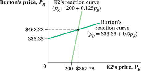
Consider our example of the two snowboard manufacturers, Burton and K2. We just determined that at the Nash equilibrium for these two firms, each firm produced 600 snowboards at a price of $300 per board. Now let’s suppose that Burton launches a successful advertising campaign to convince snowboarders that its product is superior to K2’s so that the demand for Burton snowboards rises to qB = 1,000 – 1.5pB + 1.5pK, while the demand for K2 boards falls to qK = 800 – 2pK + 0.5pB. (For simplicity, assume that the marginal cost is still zero for both firms.)
Derive each firm’s reaction curve.
What happens to each firm’s optimal price?
What happens to each firm’s optimal output?
Draw the reaction curves in a diagram and indicate the equilibrium.
Solution:
To determine the firms’ reaction curves, we first need to solve for each firm’s marginal revenue curve:
MRB = 1,000 – 3pB + 1.5pK
MRK = 800 – 4pK + 0.5pB
By setting each firm’s marginal cost equal to marginal revenue, we can find the firm’s reaction curve:
MRB = 1,000 – 3pB + 1.5pK = 0
3pB = 1,000 + 1.5pK
pB = 333.33 + 0.5pK
MRK = 800 – 4pK + 0.5pB = 0
4pK = 800 + 0.5pB
pK = 200 + 0.125pB
We can solve for the equilibrium by substituting one firm’s reaction curve into the other’s:
pB = 333.33 + 0.5pK
pB = 333.33 + 0.5(200 + 0.125pB ) = 333.33 + 100 + 0.0625pB
pB = 433.33 + 0.0625pB
0.9375pB = 433.33
pB = $462.22
We can then substitute pB back into the reaction function for K2 to get the K2 price:
pK = 200 + 0.125pB
= 200 + 0.125(462.22) = 200 + 57.78 = $257.78
452
So, the successful advertising campaign means that Burton can increase its price from the original equilibrium price of $300 (which we determined in our initial analysis of this market) to $462.22, while K2 will have to lower its own price from $300 to $257.78.
To find each firm’s optimal output, we need to substitute the firms’ prices into the inverse demand curves for each firm’s product. For Burton,
qB = 1,000 – 1.5pB + 1.5pK = 1,000 – 1.5(462.22) + 1.5(257.78)
= 1,000 – 693.33 + 386.67 = 693.34
For K2,
qK = 800 – 2pK + 0.5pB = 800 – 2(257.78) + 0.5(462.22) = 800 – 515.56 + 231.11 = 515.55
Burton now produces more snowboards (693.34 instead of 600), while K2 produces fewer (515.55 instead of 600).
The reaction curves are shown in the diagram below:

Application: Computer Parts—Differentiation Out of Desperation
Bertrand competition with identical products is extremely intense. In equilibrium, firms set price equal to marginal cost and earn no profit. This is a situation that most firms would like to avoid if they could. As we just saw, however, firms can earn profits if their products are differentiated. This gives firms a huge incentive to try to differentiate their products from their competitors’ products, even if an outsider to the market might not think there are really any important differences among them.
This sort of behavior was documented by economists Glenn Ellison and Sara Ellison in an online market for computer chips that we discussed briefly in Chapter 2.11 In this market, high-
Ellison and Ellison documented how some computer parts retailers in the market used a little economic know-
453
Just how could these firms differentiate what were otherwise identical computer chips? They couldn’t do this the way K2 and Burton can with the snowboards they sell, by varying designs, materials, and so on. So they turned to slightly more, well, creative methods—
Ellison and Ellison found that online firms rely on two primary means of obfuscation. In the first, the firm lists a cheap but inferior product that the price search engine displays at the beginning of its listings. Customers click on this product and are redirected to the firm’s Web site, where the company then offers a more expensive product upgrade. Once one firm undercuts its competitors with this “loss leader” strategy, all firms will list similarly cheap products or risk having their product listing buried deep in the last pages of the listings. As a result, it becomes more time-
Another common strategy is the use of product add-
Obfuscation methods such as these are part of the reason the Bertrand model with identical products that we first studied is so unusual in the real world. Even products that aren’t obviously differentiable can be made to stand out through some clever strategies devised by the firms selling them. Given that firms selling such products would otherwise expect to earn something close to nothing, they have a massive incentive to figure out differentiation strategies, and thus try to reduce competition. 