Expected value gives us a way to think about risks in the context of investment. But, as we see in this section, when we use expected value analysis, we are implicitly assuming that people aren’t especially afraid of risk. For example, in expected value terms, a 1% chance of $100 million is worth just as much as having $1 million in cash, even though the former is a much less certain proposition than the latter. In this section, we explore what happens when people do not like taking risks and see why insurance is valuable to these people. In addition, we learn how risk changes investment decisions.

To understand what we mean by people not liking risk, think about a person and the utility he gets from consuming the goods he can buy with his income. Our analysis in Chapter 4 explains what bundle of goods a person picks given the goods’ prices and the person’s income, but when trying to figure out consumers’ distastes for risk, we don’t need to keep track of exactly what goods are in that bundle. All we need to know is the total amount of utility this person enjoys at any given income level.

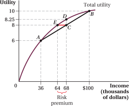
We plot the relationship between utility and income for a random guy named Adam in Figure 14.3. Adam’s income is shown on the horizontal axis, and his utility from consuming the goods he buys with that income level is on the vertical axis. Utility rises with income, as we would expect, because the more income he has, the more stuff he can buy. However, the curve becomes less steep as his income rises. That is, Adam has diminishing marginal utility of income. The bump in utility he would enjoy from an increase in income of, say, $10,000 to $15,000 is more than the extra utility he’d experience from moving from an income of $1,000,000 to $1,005,000. It turns out that if diminishing marginal utility holds, Adam will be sensitive to risk and willing to pay to eliminate or reduce uncertainty.

To make the relationship between risk and diminishing marginal utility as clear as possible, take a specific example. Suppose most of Adam’s income comes from a country store he owns, and that the only important uncertainty his business faces is whether the store is destroyed by a tornado (causing Adam’s income to take a big hit).

560

We assume the utility, U, that Adam enjoys from goods purchased with his income is given by the function

where I is Adam’s income in thousands of dollars. This utility function is plotted in Figure 14.3, and it exhibits diminishing marginal utility of income.

Now suppose that Adam’s income is $100,000 in a year there is no tornado and only $36,000 if there is a tornado. The utility levels corresponding to these incomes are shown as points B and A, respectively, in Figure 14.3. With $100,000 in income, Adam’s utility is with $36,000 in income, it’s .

Let’s say the probability of a tornado is ridiculously high, 50%, to make the math easy. This is where the uncertainty comes from.

Following a basic expected value calculation, we first compute Adam’s expected income for the year. There’s a 50% chance his store blows down, giving him an income of $36,000. There’s a 50% chance of no tornado, and his income is $100,000. Applying the formula for computing expected values, we find that Adam’s expected income is $68,000:

Expected income = (0.5 × $36,000) + (0.5 × $100,000)

= $18,000 + $50,000

= $68,000

Similarly, we can compute his expected utility:

Expected utility = (0.5 × 6) + (0.5 × 10)

= 3 + 5

= 8

We plot these expected income and utility levels at point C. Notice how this point is halfway along the straight line connecting A and B, the income-utility combinations in the tornado and no-tornado cases. This isn’t a coincidence. Adam’s expected income and utility values will be somewhere on that same line for any probability of a tornado. Where exactly on the line the point will be depends on the probability that each event (tornado or no tornado) occurs. The higher the probability of a tornado, the closer Adam’s expected income and utility will be to the tornado income-utility point A. (If a tornado happens 100% of the time, point A is the expected income and utility.) If the probability of a tornado is low, Adam’s expected income and utility will be near point B. The expected values shown at point C happen to be at the halfway point on the AB line because the tornado has a 50% chance of happening.

Notice another important thing about point C: It’s at an expected utility level, 8, that is below Adam’s utility function at that same income level. According to Adam’s utility function, an income level of $68,000 allows him to achieve a utility of , as shown at point D in Figure 14.3. What this means is that the same expected income, $68,000, can give Adam different levels of expected utility depending on the riskiness of the underlying income levels on which the expectation is based. Due to the chance of tornado, Adam’s income is uncertain, and his $68,000 in expected income delivers an expected utility of 8. But, if his income is guaranteed to be $68,000, even though his expected income of $68,000 has not changed, his expected utility would be 8.25. In other words, the very uncertainty about what his income will be reduces Adam’s expected utility. If a person prefers having a guaranteed amount to having a risky but equivalent-in-expected-value amount, we say the person is risk-averse. Uncertainty reduces the utility of a risk-averse person like Adam.

561

A related way to see how uncertainty reduces expected utility is to ask what guaranteed income would offer Adam the same expected utility level as his uncertain income. That equivalent income level, sometimes referred to as the certainty equivalent, is shown at point E in Figure 14.3. The certainty equivalent in this example is $64,000, because . Adam derives the same expected utility from a guaranteed $64,000 income as he does from having a 50% chance of a $36,000 income and a 50% chance of a $100,000 income. Another way to put this is that Adam is willing to give up $4,000 in expected income ($68,000 – $64,000) in exchange for eliminating his income uncertainty. This income difference is called the risk premium—it’s the extra amount of expected income (here, $4,000) Adam must receive to make him as well off when his income is uncertain as when it is guaranteed.

Notice how these relationships we’ve just pointed out—that for risk-averse individuals, expected utility falls as a given expected income becomes more uncertain, and that risk-averse individuals are willing to give up expected income to reduce uncertainty—are, graphically speaking, a consequence of the diminishing marginal utility of income. That is, the fact that point C (or any point on the AB line) is below the income-utility curve is a direct consequence of the fact that there is diminishing marginal utility of income. Diminishing marginal utility causes this curve to be concave as income rises, ensuring that any uncertain combination of income-utility outcomes will have an expected utility below that of an equivalent expected income that is guaranteed.

A world full of uncertainties and risk-averse people creates demand for insurance. We all understand the basic idea of insurance, but economists define it specifically as when one economic actor pays another to reduce the payer’s economic risk. The details of the insurance-risk aversion connection are important to understand, and we’ll go through them in a moment, but the basic idea is simple. If someone is risk-averse, he will pay to have his risks reduced. That’s what insurance does: It reduces risk by paying the policyholder when things would otherwise be bad (his car is stolen, he becomes sick and needs to pay a lot of medical bills, etc.). In exchange for this, the policyholder pays a premium to the insurer each year and makes do with a little less income (by the amount of the premium) in exchange for help against the possibility of something bad.

The Value of Insurance The loss in expected utility Adam experiences due to the uncertainty of his income and his willingness to give up some expected income to reduce this loss suggest a way to make him better off. Suppose someone or some company offers him an insurance contract to reduce his uncertainty and that it involves the following arrangement. If Adam’s store blows down, the insurer will pay him a sum of money. This will reduce his losses in the bad situation. In exchange, Adam makes a payment to the insurer—a policy premium—if there isn’t a tornado. This premium reduces his income in a good situation; there’s no tornado, but Adam has to do without the money he paid for the premium. By reducing Adam’s uncertainty, however, the insurance contract raises Adam’s expected utility for any given expected income level. Note that the arrangement does not raise Adam’s expected utility by increasing his expected income; in fact, the insurance policy could very well reduce his expected income. Nevertheless, he benefits because less uncertainty translates into greater expected utility.

We can see this benefit more explicitly in some examples. A straightforward policy would have the insurer pay Adam $32,000 if a tornado destroys his store, while having Adam pay the insurer a $32,000 premium if there is no tornado. Under such a policy, Adam’s income is $68,000 regardless of whether a tornado occurs. If there’s a tornado, his income is $36,000 and his payout from the insurer is $32,000, and $36,000 + $32,000 = $68,000; if no tornado occurs, his income is $100,000 and his insurance premium is $32,000, and $100,000 – $32,000 = $68,000. As we saw above, that guaranteed income of $68,000 yields Adam an expected utility of 8.25, greater than the expected utility of 8 he would receive without an insurance policy and the same expected income of $68,000. This policy offers what is sometimes called complete insurance or full insurance: All uncertainty has been eliminated for Adam; he ends up equally well off no matter what event happens (tornado or no tornado). Even partial insurance is valuable, however. Suppose that the policy instead pays Adam $20,000 if there is a tornado in exchange for a $20,000 premium in the case of no tornado. This makes his income $36,000 + $20,000 = $56,000 in the case of a tornado and $100,000 – $20,000 = $80,000 if no tornado occurs. This policy keeps Adam’s expected income at $68,000 (0.5 × $56,000 + 0.5 × $80,000 = $68,000), but gives him an expected utility of . While this is less than the expected utility of 8.25 from having a guaranteed $68,000 in income, it is higher than Adam’s expected utility of 8 without a policy.

562

Insurance is a good deal for Adam, but what’s in it for the insurer? An insurance policy basically shifts Adam’s risk to the insurer: The insurer does not know for certain what its profit from the policy will be. However, insurers don’t typically suffer a loss as a result of this transfer because they issue a large number of policies like Adam’s. By adding together all these risks from all the policies they issue, insurers greatly reduce the uncertainty of their profits.

To see why adding risks together helps an insurer, suppose that an insurer has sold policies to thousands of people exactly like Adam, each of whom owns a store that delivers income to the storeowner but also has a 50% chance of blowing down. Although it is uncertain if any particular store is going to blow down, because the insurer covers thousands of such stores, in a given year that insurer can expect almost exactly half of its covered stores to blow down. Thus, rather than having high uncertainty over the claims it will have to pay, the insurer actually has low uncertainty. The insurer doesn’t make big profits half the time and lose big money the other half; instead, it knows it’s going to almost surely have to pay claims on about half its stores while collecting premiums from the other half. This diversification—reducing risk by combining uncertain outcomes—is one of the key functions of insurance markets. An important part of making diversification work is that risks being added together must be at least partially unrelated. If instead they were highly correlated with one another—for instance, if all the insured stores were tightly packed together in the same location so that if one blew down, they all would—the insurer couldn’t diversify away the risk. Half the time no stores would blow down, and half the time all the stores would blow down. The insurer would be left with a risk just as uncertain as Adam’s, but bigger in financial terms.

Insurers can benefit from offering to take away policyholder’s risks in another way. Remember that risk aversion creates a willingness to pay to remove or reduce risk. Insurers can design policies to capture some of this value. Both of the example policies we discussed above have the same expected profit for the insurer: zero. The payment the insurer makes to Adam in case of a tornado equals the policy premium he pays in the absence of a tornado, and both outcomes happen with equal probability. (For example, 0.5 × –$32,000 + 0.5 × $32,000 = –$16,000 + $16,000 = $0.) When the expected net payments of an insurance policy total zero—that is, when the expected premiums equal the expected payouts—a policy is said to be actuarially fair.

But, we’ve just seen how insurance has value for consumers like Adam; in real life, insurers design policies to capture some of this value. Consider the following policy: The insurer pays Adam $20,000 if there is a tornado, while Adam pays a $24,000 premium if no tornado occurs. Adam’s expected utility under this policy is . The policy raises his expected utility relative to the level it would be without the policy. Adam’s expected income under the policy is (0.5 × $56,000) + (0.5 × $76,000) = $66,000. This is $2,000 less than his expected income of $68,000 without the policy, but Adam is willing to give up this $2,000 because his expected utility is higher with the policy than without it. As we saw above, in fact, Adam is willing to give up as much as $4,000 in expected income to purchase a policy that would remove all of his income uncertainty.

563

From the insurer’s point of view, Adam’s $2,000 drop in expected income is its expected profit from the policy: There is a 50% chance it will have to pay Adam $20,000 and a 50% chance it will not have to pay Adam anything, but will earn a $24,000 premium, yielding an expected profit of (0.5 × $24,000) – (0.5 × $20,000) = $2,000. While this outcome from Adam’s policy is uncertain, again, if the insurer sells thousands of such policies to unrelated risks, it can expect to earn profits of nearly $2,000 per policy without much uncertainty around that total.7

Why would the insurer design a policy that only has an expected profit of $2,000 when Adam would give up as much as $4,000 in expected income for insurance? Well, the insurer can only charge the higher premium if the market isn’t competitive. The more competition, the more the terms of policies will be tilted in the favor of policyholders and toward being actuarially fair.

564

Given the connection between diminishing marginal utility of income (reflected in how curved the utility-income relationship is) and risk aversion, it should be clear that the greater the curve in a consumer’s utility function, the more risk-averse he is.

Figure 14.4 demonstrates this in an example. The figure’s two panels show portions of the utility-income functions for two consumers with different degrees of curvature. The consumer in the left panel (a) has relatively little curvature; his marginal utility of income drops relatively slowly as his income rises. The consumer in the right panel (b) has a relatively large amount of curvature and a marginal utility of income that falls quickly as his income rises.

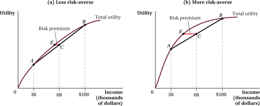
Suppose that these consumers faced a situation like Adam’s, with a 50% chance of a $36,000 income and a 50% chance of a $100,000 income. The utility-income points corresponding to these outcomes are shown at points A and B in both panels. The consumers’ expected incomes and utilities again occur at the midpoints of the AB lines, point C in each panel. The figure also shows the certainty equivalents for the consumers, point E.

The horizontal distances between points C and E in each panel—that is, the expected income consumers are willing to give up in order to have their risky expected incomes at point C replaced by the guaranteed income at point E—are the consumers’ respective risk premia. Notice how the risk premium of the more risk-averse consumer in the right panel is larger than that for the less risk-averse consumer. This reflects the fact that the degree of a consumer’s risk aversion is tied to the curvature in his utility function (or equivalently, the rate at which his marginal utility of income falls as his income grows). When there is more curvature, the expected utility loss due to any given amount of income uncertainty is larger. Consumers with highly curved utility functions have a greater willingness to pay to have risk reduced.

565

566

If the curve stays straight, we call the consumers risk-neutral. If it curves up (which can happen), then we say that person is risk-loving. A risk-lover would actually pay money to have a chance to gamble on a big payoff rather than take the certainty equivalent.

567