17.2 Correcting Externalities
Left to its own devices, a free market with externalities produces more than (if the externalities are negative) or less than (if the externalities are positive) the optimal welfare-
Is society doomed to live with this inefficiency? Not necessarily. Just as we saw in Chapter 16 that asymmetric information’s potential welfare losses offer powerful incentives to create institutions that remedy them, the same is true for externalities. Governments or the economic actors in markets with externalities may implement one of several interventions that can reduce the inefficiencies externalities create.
Externality fixes come in two basic types: those that work through their effect on price and those that work through their effect on quantity. Both types try to steer the market away from the inefficient outcome of the private market (in which only private marginal costs and benefits are considered) toward the more efficient outcome (in which social marginal costs and benefits are considered). The price approach pushes prices to reflect the true social costs and benefits. The quantity approach pushes quantities toward efficient levels.
Because many real-
The Efficient Level of Pollution
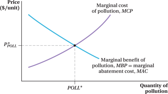
efficient level of pollution
The level of emissions necessary to produce the efficient quantity of the good tied to the externality.
Before considering how to correct for an externality, we need to consider how the government chooses its efficiency target. The goal is to set the level of total pollution allowable at its efficient level. The efficient level of pollution is the level of emissions necessary to produce the efficient quantity of the good tied to the externality. Therefore, the total amount of emissions allowable is set at the level that allows the market for the good to produce the quantity at which demand equals marginal social cost.
We can also think about the efficient amount of pollution (or any negative externality) as the level that balances its costs and benefits. Pollution’s costs—
We can see how the efficient level of pollution is determined in Figure 17.3. In reality, it is likely that the marginal cost of pollution (MCP) rises with the level of pollution. The incremental damage of more pollution is relatively modest at low levels, but the severity of the damage grows as pollution increases. This is reflected in the shape of curve MCP in Figure 17.3.
660
The marginal benefit of pollution (MBP), on the other hand, is likely to be high at low levels because some positive level of pollution is necessary to make goods. But, the marginal benefit will tend to fall as pollution output increases (and as output of the good increases). At higher output levels of pollution (and the good), production technologies can become more flexible so that less pollution is produced at higher quantities of the good’s output. Also, because demand curves slope down, the price at which an industry can sell its marginal unit of output falls, which, in turn, makes pollution less valuable on the margin. These factors are reflected in curve MBP in Figure 17.3.
marginal abatement cost (MAC)
The cost of reducing emissions by 1 unit.
There is a different way to think about the marginal benefit curve MBP that allows us to consider how much it would cost a firm to reduce the level of pollution it creates. Just as the MBP curve shows the marginal benefit from pollution, it also reflects the flip-
The efficient level of pollution is where its marginal benefit equals its marginal cost, or POLL* in Figure 17.3. The logic is the same as we’ve seen before: If something’s marginal benefit is higher than its marginal cost, produce more; if its marginal cost is greater than its marginal benefit, produce less. Net benefits are maximized where the next unit equates the two marginal effects.
If we want to think of the marginal benefit curve as being the marginal abatement cost curve instead, we can interpret optimal pollution in terms of emissions cuts. Emissions should be cut whenever the marginal cost of a reduction in the level of emissions (as reflected by the MAC curve) is less than the reduced harm (as reflected by MCP). This will be true at any pollution levels greater than POLL*. On the other hand, if marginal abatement costs are greater than the marginal cost of the pollution, which will be the case at pollution levels less than POLL*, then pollution cuts should be scaled back. These considerations are balanced at the optimal pollution level POLL*.
661
The optimal “price” of pollution is equal to the marginal cost of pollution (and marginal benefit) at the optimal quantity, or P*POLL in Figure 17.3. If pollution were tradable (which, as we see later, it can be), at P*POLL polluters would be willing to purchase the right to pollute up to the level POLL*. For levels of pollution below POLL*, the price P*POLL is lower than the value from being able to pollute more (measured by the marginal benefit of pollution). At the same time, those harmed by pollution would still be willing to sell an amount of pollution rights equal to POLL*, because at this price they are being more than compensated for the harm they suffer (P*POLL > MCP).
In principle, an efficient level of pollution could result from either price or quantity mechanisms. If regulators could impose the socially optimal price in a market, for instance, the quantity (of either the good or the externality) at that price would also be at its optimal level. Similarly, if regulators could specify the socially optimal quantity, the price at that quantity would be the optimal price. In practice, however, we will see that one approach may be easier than the other to enact, depending on the nature of the externality and the information available to regulators.
Using Prices to Correct Externalities
One way to view the failure of the free market in the presence of externalities is that the market participants do not consider the correct, society-
For goods tied to negative externalities, price-
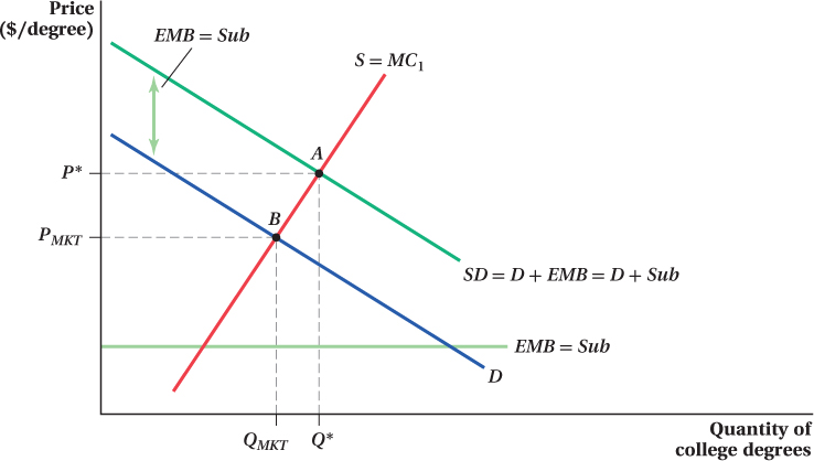
For goods associated with positive externalities, additional demand can be added by paying firms for producing (or buyers for purchasing) each unit of output. This, in essence, raises the demand curve faced by the producers, spurring them to increase output. Therefore, the price received by the seller and the amount of output produced will become equal to their efficient levels.
Pigouvian tax
A tax imposed on an activity that creates a negative externality.
Pigouvian Taxes One of the most common types of price-
Let’s look at how a Pigouvian tax works. Suppose that coal-
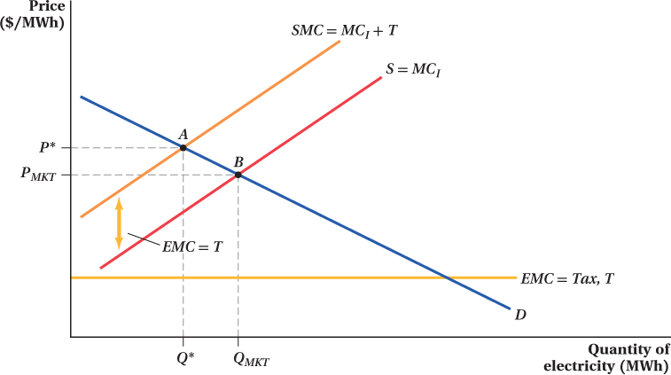
662
Because the electricity industry’s private marginal costs MCI are not the same as the social marginal costs SMC, we get overproduction: The power company generates QMKT when the optimal quantity is Q*.
Now, let’s say that a government could impose a tax T per MWh on electricity production equal to the external marginal cost EMC of pollution. This would increase the private marginal cost of supplying energy, and shift MCI up to MCI + T. Because T = EMC, the industry’s marginal cost curve is now the same as the social marginal cost curve SMC. The old marginal cost curve MCI intersected the demand curve at the price PMKT. At that price, the industry’s output was QMKT. If the size of the tax is chosen so that the tax-
The Pigouvian tax raises the electricity industry’s marginal cost by an amount equal to the external damages its production causes. This exactly aligns the industry’s private incentives with society’s. In effect, the Pigouvian tax “internalizes” the pollution externality. That is, it forces the industry to take into account the external damage of its operations when it decides how much electricity to generate. This process results in the efficient market outcome.
In reality, there are all kinds of Pigouvian taxes. One of the rationales for placing taxes on cigarettes and alcohol and for the recent calls for imposing taxes on soda arises from the external costs (from second-
Another example of a Pigouvian tax comes from the European Union. A few years ago, the EU proposed curbing greenhouse gas pollution and global warming by imposing a carbon emissions fee on international airline flights. This fee would force the airlines to account for the high amounts of greenhouse gas emissions made by large commercial aircraft. The effectiveness of this fee suffered when several large nations including India and China refused to require their airlines to pay it.
663
Application: Facebook Fixes an Externality
In February 2012 a business that published an unpaid post on Facebook via its Pages account could expect about 16% of its fans to see the post. By November 2014, however, a business would be happy with a 2% showing. Facebook offers Pages accounts to allow businesses, brands, and organizations to share information and connect with a fan base at no cost. But over time these connections have reached fewer and fewer fans. In Facebook lingo, “organic reach,” or number of unique visitors per post, has declined.
Why this drop in Pages’ reach? One reason is increased competition—
Facebook has spent a lot of time figuring out what its users value, and it has found that users don’t want to see certain types of posts by Pages. For instance, users don’t like explicit requests to “like,” “comment,” or “share” a post (practices sometimes called “like-
Because these attributes were experienced as bads only by users and not by the post’s publishers (Pages managers care about maximizing a post’s visibility regardless of its quality), like-
Why is Facebook so concerned with making the reach of the newsfeed more efficient (or, in Mark Zuckerberg’s words, “build[ing] the perfect, personalized newspaper for every person in the world”)? Because, on a larger scale, Facebook, like its users, suffers from the negative externalities: Bad posts turn off users and decrease Facebook’s ad revenue. Unlike users, however, Facebook has a say in how many low-
Pigouvian subsidy
A subsidy paid for an activity that creates a positive externality.
Pigouvian Subsidy When there is a positive externality, a Pigouvian subsidy can be used to decrease a good’s price (paid by the buyer) to take into account the external marginal benefits. The subsidy raises the effective price (the market price plus the subsidy) at which producers can sell their products, thus making it profit-
664
There are many types of actual subsidies that are at least supposed to be based on Pigouvian principles. Tax credits for education or to buy hybrid cars and fuel-
One practical problem facing Pigouvian taxes and subsidies is how to figure out their correct size. Realistically, it’s difficult to estimate the exact external marginal cost of carbon pollution or the exact external marginal benefit from more college degrees, so setting the correct rate for the Pigouvian tax or subsidy is also difficult. If a government sets the Pigouvian tax or subsidy at the incorrect level, the market price and quantity will still be inefficient. We discuss this problem more below.
figure it out 17.2
For interactive, step-
Refer to Figure It Out 17.1. Suppose the government places a $0.50 tax on each ream of paper sold.
What price would buyers pay, and what price would sellers receive (net of the tax)?
How many reams of paper would be sold?
Solution:
To solve this problem, we can use the method we learned in Chapter 3, where we consider that the price paid by buyers, PB, is equal to the price received by sellers, PS, plus the tax: PB = PS + T. Therefore, PB = PS + 0.50. We can rewrite the demand curve and the supply curve (the industry marginal cost curve) from Figure It Out 17.1:
QD = 5 – 0.125PB and QS = 0.5PS
Because PB = PS + 0.50, we can substitute this expression into the demand curve for PB:
QD = 5 – 0.125PB = 5 – 0.125(PS + 0.50) = 5 – 0.125PS – 0.0625 = 4.9375 – 0.125PS
Now that the supply and demand equations are both written in terms of PS, we can solve QD = QS:
4.9375 – 0.125PS = 0.5PS
0.625PS = 4.9375
PS = $7.90
PB = PS + 0.50 = $7.90 + $0.50 = $8.40
Note that this is the socially optimal price we found in Figure It Out 17.1.
To solve for the quantity sold, we can substitute the buyer’s price (PB = $8.40) into the demand curve or the seller’s price (PS = $7.90) into the supply curve:
QD = 5 – 0.125PB = 5 – 0.125(8.4) = 5 – 1.05 = 3.95
QS = 0.5PS = 0.5(7.9) = 3.95
This is the socially optimal quantity.
665
Application: Would Higher Driving Taxes Make Us Happier Drivers?
Imagine you were the only driver on the road. You could go fast, ignore stop lights and stop signs, and make left turns without first checking for oncoming traffic—
In 2003 former London Mayor Ken Livingstone looked at the externalities associated with driving in his city and decided they were way too high. Over 1 million people commuted into the city center during the peak morning rush hour alone. While the city offered public transit, too few people used it. As a result, commuting on the roadways in London—
Mayor Livingstone used economics to try to solve the problem by instituting a Pigouvian tax on drivers. Starting in 2003, drivers entering London’s central district faced a £5 toll. Estimates made before the fee was levied suggested that Londoners would pay about £286 million in tolls, but would see about £331 million in savings in time and vehicle operation costs. In the first year of the tax, congestion was reduced by an estimated 30%. Cars were traveling at speeds unheard of since the 1960s—
666
The biggest benefit of fewer cars on the road, surprisingly, might not be less congestion or less pollution. In fact, economists Aaron Edlin and Pinar Karaca-
Tolls are one way to deal with an automobile externality; gasoline taxes are another. When the gas tax is raised, the price of gas increases and people choose to drive less often. Edlin and Karaca-
Quantity Mechanisms to Correct Externalities
Quantity-
quota
A regulation mandating that the production or consumption of a certain quantity of a good or externality be limited (negative externality) or required (positive externality).
Quotas The simplest of the quantity-
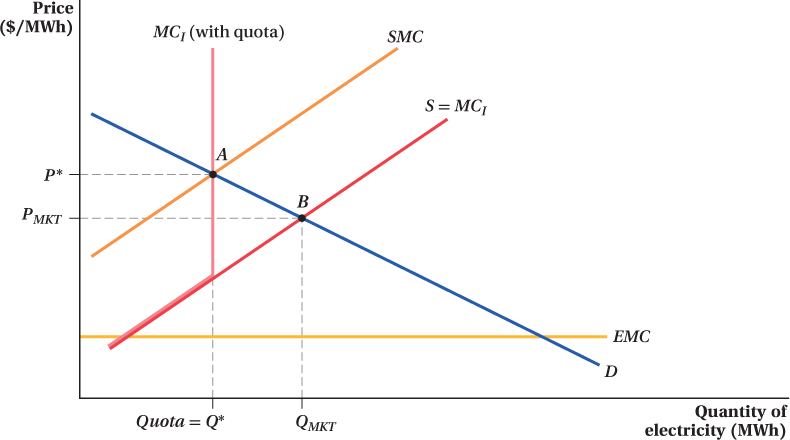
In Figure 17.6, we look once again at the market for electricity production and see that the pollution externality leads to excessive production at QMKT and an inefficient market outcome. Suppose that the government enacts a law mandating that the production of electricity can be no greater than Q*. With this law in place, the private MCI curve becomes vertical at that quantity level. The private MCI curve now intersects the demand curve at point A and the private decision matches the socially efficient one.
Examples of quotas used in actual practice include restrictions on the amount of pollution factories can emit and the amount of noise neighbors can make. Similarly, hunting and fishing licenses limit the number of fish or animals a person can take because of the negative externality of overfishing and overhunting.
We see fewer real-
667
Practically speaking, however, the use of quotas creates complications. First, as with setting Pigouvian taxes, it is difficult to determine what the socially optimal amount of the quotas actually should be.
A second difficulty with quotas is that the government often wants to influence the total amount of an externality produced by an industry, but can only set quotas on a firm-
Third is the question of the distribution of costs and benefits. A Pigouvian tax, for example, generates revenues for the government (or costs the government in the case of subsidies). With quotas and mandates, the benefits or costs are left with the market participants. With licensing, the government receives some revenue, while market participants incur some cost but also reap some benefits.
Government Provision of a Good Another type of quantity intervention in the case of positive externalities occurs when the government actually provides the product itself. Basic scientific research has a large positive externality and little private sponsorship, so the federal government subsidizes it through tax credits and research funding. Governments also perform research directly, as does the United States at the National Institutes of Health and a system of federal labs around the country.
Price-Based versus Quantity-Based Interventions with Uncertainty
668
We saw above that, as a matter of principle, quantity and price mechanisms can be equally effective at addressing externalities. In reality, though, there are situations in which one type of market intervention might be preferred to the other.
A particularly important situation in which one mechanism might be preferred to the other is when the optimal level of the externality is not fully known. The importance of uncertainty in dealing with externalities was first pointed out by American economist Martin Weitzman in 1974.12
Such uncertainty is common. The marginal benefits and the marginal costs of pollution are difficult to measure and often shift with changes in technologies, input costs, and new discoveries about how damaging pollution is to human health. As a result, efforts to intervene in markets with externalities are generally inexact, so any Pigouvian taxes or quantity mandates that regulators set are not exactly right. Not being exactly right is always costly, but it can be even more costly if the wrong intervention is used.
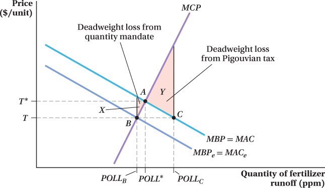
Let’s look at Figure 17.7, which illustrates the marginal cost and marginal benefit of water pollution caused by fertilizer runoff from farms (measured in parts per million, or milligrams per liter of water). The marginal cost of water pollution is shown by the MCP curve. The marginal benefit of pollution and the marginal cost of removing this pollution are shown by the MBP = MAC curve. In Figure 17.7, the efficient quantity of runoff pollution in the market POLL* is found where the marginal benefit of pollution is exactly equal to the marginal cost of pollution (point A).
669
Before we examine how uncertainty can affect the ability of a regulation to move the market to its efficient level of pollution, let’s remind ourselves of how to measure the deadweight loss that occurs when the pollution level is not at the efficient level. The deadweight loss equals the area between the marginal benefit of pollution (alternatively, the marginal abatement costs) and the marginal cost of pollution for each of the units of pollution between the efficient level of pollution and the current level of pollution.
If the level of pollution is too high (to the right of POLL*), pollution costs society more (as seen by the MCP curve) than its value (in terms of output produced along with the pollution, reflected in the MBP curve). Conversely, when the level of pollution is inefficiently low (the level lies to the left of POLL*), there are units of pollution that provide greater value (in terms of the output that would be produced along with the pollution) than their cost.
Now suppose the regulator does not know exactly what farmers’ marginal abatement costs are, and so is unsure about the true marginal benefits of water pollution. Can we say whether the regulator would be better off choosing a quantity-
For example, suppose the regulator mistakenly estimates farmers’ marginal abatement costs as being lower than they really are, shown by curve MBPe = MACe in Figure 17.7. If these were the true abatement costs, the optimal level of pollution would be POLLB because the marginal cost of pollution is equal to the estimated marginal benefit of pollution at point B. The regulator could achieve a pollution level of POLLB in two ways: by limiting the quantity of fertilizer used so that total runoff pollution is POLLB, or by setting a tax on runoff at price T.
If the regulator uses a quantity mechanism, the amount of pollution will be limited to POLLB, lower than the socially optimal level POLL*. In this case, the deadweight loss from incorrectly mandating the quantity is the triangle X in Figure 17.7. This area reflects the pollution for which the true marginal benefit is higher than the marginal cost to society. This pollution does not occur, however, because of the quantity restriction at the wrong pollution level.
If the regulator instead uses a Pigouvian tax equal to T, farmers will reduce their fertilizer use from where it would be without any tax until their marginal abatement cost equals the tax (at point C). Additional cuts in the level of pollution beyond this point would be more expensive (in terms of forgone output) than simply paying the pollution tax. So, this incorrect tax (due to the mis-
This result—
The reason why the deadweight losses are so much larger with price mechanisms results from the way we set up the example. We’ve drawn the marginal abatement curve as relatively flat and the marginal cost of pollution curve as relatively steep. The flat MAC curve implies that farmers’ abatement choices are very sensitive to the price of abatement (in other words, the tax), so being just a little wrong on setting a Pigouvian tax leads to wild swings in the amount of pollution the farmers create. These large swings, in turn, cause big inefficiency losses because the marginal cost of pollution is so sensitive to the amount of pollution (as shown by the steep MCP curve). Therefore, when faced with cases in which farmers’ abatement choices are sensitive to a tax and the marginal cost of pollution is likely to rise rapidly with pollution, regulators should favor quantity-
670
If the situation were reversed, and the marginal abatement cost curves were fairly steep and the marginal cost of pollution curve were relatively flat, price mechanisms cause fewer inefficiency losses than quantity-
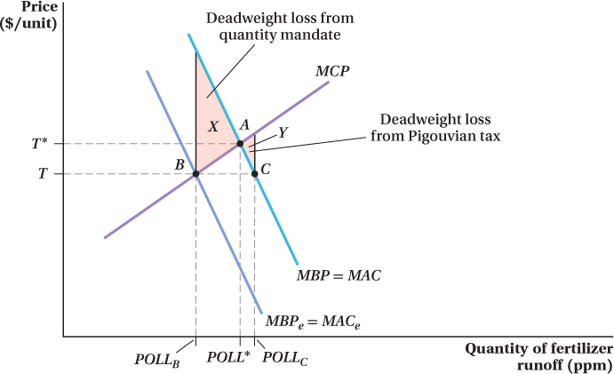
In Figure 17.8, the optimal level of pollution from fertilizer runoff is at point A, where the marginal cost of pollution equals the marginal benefit of pollution (or marginal abatement cost), and the efficient level of pollution is POLL*. Once again, suppose the regulator believes that farmers’ abatement costs are lower than they really are, shown by curve MBPe = MACe. If regulators use a quantity-
Figure 17.8 shows that when the marginal abatement cost curve is steep relative to the marginal cost of pollution curve, setting incorrect Pigouvian taxes is less costly than setting incorrect quantity mandates. The relative insensitivity of abatement to the level of the tax means that being a little wrong about the optimal tax won’t have much effect on the actual level of pollution. But, setting the wrong quantity will be very costly. Regulations that force producers to undertake unnecessarily high abatement will be expensive relative to the marginal costs of pollution it saves. Similarly, mandating too little abatement will mean that some pollution cuts with benefits that would far outweigh their costs won’t be made.
671
Therefore, when regulators are uncertain about the optimal level of an externality, the choice of quantity-
A Market-Oriented Approach to Reducing Externalities: Tradable Permits Markets
Trying to mandate the total externality in a market by restricting each firm’s quantity or determining the correct amount to tax involves a lot of effort. Worse, it may lead to costly errors if producers differ in their costs of changing output levels. It would be optimal for firms that could do this more cheaply to make a larger share of the necessary quantity adjustments. But, it can be very difficult for a regulator to know what each firm’s costs are and set quantity restrictions or taxes appropriately.
tradable permit
A government-
In these cases, it can be preferable to allow firms to jointly determine how best to reduce an externality to its optimal level. Tradable permits for pollution can achieve this. These are permits issued to firms by the government that allow the holder to emit a certain amount of pollution, and no one can pollute without one. After the permits are allocated among firms, they can be traded, allowing some firms to emit a greater amount of pollution than others. In essence, a market for pollution emissions develops. Such systems are sometimes called “cap-
A competitive tradable permits market will arrive at a price per permit that equates the marginal cost of pollution abatement across all firms. Suppose the permit price was above a firm’s marginal abatement cost (alternatively, its marginal benefit of polluting). It could then make a profit by reducing its pollution by 1 unit and selling the permit that the marginal unit of pollution would have required. If permit prices were instead below its marginal benefit of pollution, it could raise its profits by buying a permit and polluting an extra unit. Only when the permit price equals the marginal abatement cost of the firm would it not want to change its pollution level. Because this logic holds for every firm, each firm’s level of pollution must equate that firm’s marginal abatement cost to the permit price. (This is similar to the logic in a perfectly competitive market where all firms produce a quantity that equates their marginal cost to the output price.)
This is an important result; it means the total amount of abatement in the industry (as set by the government cap) is done efficiently. If one firm has a lower marginal abatement cost than another, it should reduce pollution more. A permit market ensures that all firms have the same marginal abatement cost, so no reshuffling of pollution reduction across firms would lower the total cost of reducing pollution.
Moreover, if the government sets the total number of permits to the efficient level of pollution, then (by definition of the efficient level) the permit price will equal the marginal benefit of pollution reduction. Therefore, a competitive permit market ends up with each firm cutting pollution to the point where its cost of doing so equals society’s benefit from those cuts.
672
The permit market achieves the total emissions cuts necessary for efficiency at the lowest possible cost, and it does so without the regulator having to determine which firm cuts how much. It works because allowing permit trading lets firms that face lower abatement costs shoulder more of the emissions-