5.4 The Impact of Changes in Another Good’s Price: Substitutes and Complements
The two preceding sections showed how a change in the price of a good leads to a change in the quantity demanded of that same good. In this section, we look at the effects of a change in a good’s price on the quantity demanded of other goods.
The approach to examining what happens when the price of another good changes is similar to that in the previous sections. We start with a fixed level of income, a set of indifference curves representing the consumer’s preferences, and initial prices for the two goods. We compute the optimal consumption bundle under those conditions. Then, we vary one of the prices, holding everything else constant. The only difference is that as we vary that price, we focus on how the quantity demanded of the other good changes.
A Change in the Price of a Substitute Good
Figure 5.15 shows an example of the effects of a change in the price of a substitute good. Initially, the consumer’s utility-maximizing bundle is 15 quarts of Pepsi and 5 quarts of Coke—the point labeled A. When the price of Pepsi doubles, the consumer can only afford a maximum of 10 quarts instead of 20. The maximum quantity of Coke the consumer can buy stays at 20 because the price of Coke has not changed. As a result, the budget constraint rotates inward to BC2. In the new optimal consumption bundle B, the consumer demands more Coke (10 quarts) and less Pepsi (5 quarts).
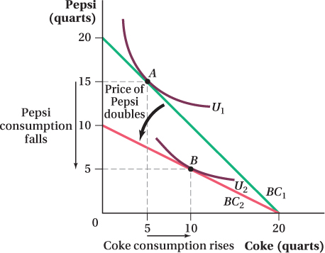
Figure 5.16: Figure 5.15 When the Price of a Substitute Rises, Demand Rises
Figure 5.16: At the original prices, the consumer consumes 15 quarts of Pepsi and 5 quarts of Coke at the utility-maximizing bundle A. When the price of Pepsi doubles, the consumer’s budget constraint rotates inward from BC1 to BC2. At the new optimal consumption bundle B, the consumer decreases his consumption of Pepsi from 15 to 5 quarts and increases his consumption of Coke from 5 to 10 quarts. Since the quantity of Coke demanded rose while the price of Pepsi rose, Coke and Pepsi are considered substitutes.
A good that can be used in place of another good.
As we learned in Chapter 2, when the quantity demanded of one good (Coke) rises when the price of another good (Pepsi) rises, the goods are substitutes. More generally, the quantity a consumer demands of a good moves in the same direction as the prices of its substitutes. The more alike two goods are, the more one can be substituted for the other, and the more responsive the increase in quantity demanded of one will be to price increases in the other. Pepsi and Coke are closer substitutes than milk and Coke.
Changes in the prices of a good’s substitutes lead to shifts in the good’s demand curve. When a substitute for a good becomes more expensive, this raises the quantity demanded of that good at any given price level. As a result, the demand curve for the good shifts out (the demand for that good increases). When a good’s substitutes become cheaper, the quantity demanded at any given price falls, and the good’s demand curve shifts in.
A good that is purchased and used in combination with another good.
When the quantity consumed of a good moves in the opposite direction of another good’s price, they are complements. Complements are often goods that the consumer would use in tandem, like golf clubs and golf balls, pencils and paper, or home theater systems and installation services. Vanilla ice cream and hot fudge, for example, are complementary goods. Figure 5.16 shows how an increase in ice cream’s price leads to a decrease in the quantity demanded of hot fudge. The higher ice cream price causes the budget constraint to rotate in, shifting the utility-maximizing bundle from A (30 quarts of hot fudge and 20 gallons of vanilla ice cream) to B (20 quarts of hot fudge and 15 gallons of vanilla ice cream). The quantity demanded of both goods falls; an increase in the price of ice cream causes the consumer to demand not only less ice cream (this is the own-price effect we’ve studied so far in this chapter), but also less hot fudge, the complementary good, as well.
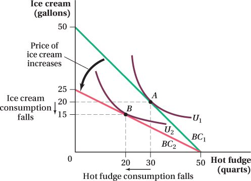
Figure 5.17: Figure 5.16 When the Price of a Complement Rises, Demand Falls
Figure 5.17: At the original prices, the consumer consumes 20 gallons of ice cream and 30 quarts of hot fudge at the utility-maximizing bundle A. When the price of ice cream increases, the consumer’s budget constraint rotates inward from BC1 to BC2. At the new optimal consumption bundle B, the consumer decreases his consumption of ice cream from 20 to 15 gallons and likewise decreases his consumption of hot fudge from 30 to 20 quarts. Since the quantities demanded of both ice cream and hot fudge decreased with an increase in price of only one of those goods, ice cream and hot fudge are considered complements.
When the price of a complement of a good increases, the quantity demanded of that good at every price decreases and its demand curve shifts in. If the price of a complement of a good falls, the quantity demanded of that good rises at all prices and the demand curve shifts out. Changes in the price of a complementary good shift the demand curve for the other good. Changes in a good’s own price cause a move along the same demand curve.
The effects of price changes in substitute and complementary goods on demand are summarized in Figure 5.17.
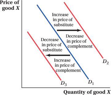
Figure 5.18: Figure 5.17 Changes in the Prices of Substitutes or Complements Shift the Demand Curve
Figure 5.18: When the price of a substitute good rises or the price of a complement falls, the demand curve for good X shifts out. When the price of a substitute good falls or the price of a complement rises, the demand curve for good X shifts in.
Indifference Curve Shapes, Revisited
As we touched on in Chapter 4, the shape of indifference curves is related to whether two goods are substitutes or complements. The more curved the indifference curve, the less substitutable (or, equivalently, the more complementary) are the goods.
In Section 5.3, we learned that the size of the substitution effect from a change in a good’s own price was larger for goods with less-curved indifference curves (see Figure 5.11). The logic behind this is that, because the marginal rate of substitution (MRS) doesn’t change much along straighter indifference curves, a given relative price change will cause the consumer to move a longer distance along his indifference curve to equate his MRS to the new price ratio. This logic holds true when it comes to the effects of changes in other goods’ prices. All that matters to the substitution effect are the relative prices; whether it’s good A’s or good B’s price that changes doesn’t matter. Therefore, an increase in a good’s price will create a larger movement toward a substitute good when the indifference curves between the goods are less curved. (A decrease in a good’s price will create a larger movement away from the substitute good.)
Application: Movies in a theater and at home—substitutes or complements?
If you own a movie theater company, one of the most important issues you face for the long-run viability of your firm is whether watching a movie on a home theater system and seeing a film in your movie-plex are substitutes or complements. Improvements in home electronics like large-screen, high-definition TVs, streaming video, and compact surround sound audio systems have greatly reduced the price of having a high-quality movie-watching experience at home. A middle-class family today can buy a home theater system that a multimillionaire could have only dreamed about a few decades ago. If movies at home are a substitute good for movies in a theater, this price reduction will reduce the number of people visiting their local movie-plex. This change will surely lead to some theaters going out of business sooner or later. If movies at home are instead a complement, theater-going will increase and bring newfound growth to the movie exhibition business.
Either case is plausible. On one hand, there is clear scope for substitution. If home electronics can better replicate the theater experience, people could find it less costly (in terms of either direct expenditures, convenience, or both) to watch a movie at home. On the other hand, if people become more interested in films in general because they now watch more at home—perhaps they develop a movie habit, or appreciate the art of film, or get caught up in following their favorite actors or watching their favorite movie again and again—then they might be more likely to see movies in theaters than they were before, particularly if theaters offer some component of the movie-watching experience that you can’t get at home (audiences with whom to laugh or be scared, really big screens, super-greasy popcorn, etc.).
The trends in the latest data don’t look promising for theater companies. Figure 5.18 shows total U.S. box office sales receipts (inflation adjusted to 2014 dollars) and the number of tickets sold per capita from 1980 to 2014.7 Total box office rose over the period, but it topped out in 2002 after a run-up in the 1990s. The decline between 2002 and 2014 was 14%, fairly substantial. The data on the number of tickets sold per capita—you can think of this as the average number of times a person goes to see a movie during the year—also peaked in 2002, but since then there has been an even more pronounced drop than in total box office. By 2014 tickets per capita had fallen below 4 movies a year, down 27% from 2002 and even below their 1980 level.
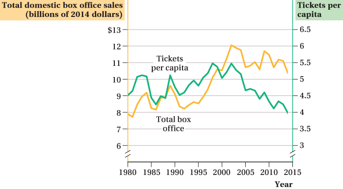
Figure 5.19: Figure 5.18 U.S. Total Box Office and Tickets Sold per Capita, 1980–2014
Figure 5.19: The overall trend in total box office sales was upward over the period and peaked in 2002. The number of tickets sold per capita also peaked in 2002, but saw more substantial declines afterward. These more recent trends suggest that home theaters might be an important substitute for movie theaters.
The decrease in theater-going after 2002 suggests that watching movies at home is a substitute, because it coincides with the period of the increased availability of big-screen HDTVs, disc players, and, more recently, streaming video. However, the data are fairly noisy: That is, there is a large amount of variation across the years, so it may be a few more years before it’s completely clear if these are long-run trends or just temporary blips due to the quality of movies or changes in the prices of other entertainment goods such as video game systems.
One bit of hope to hang onto if you’re a theater owner is that the widespread diffusion of VCRs, DVD players, and early surround-sound systems in the 1980s and 1990s didn’t permanently scar the movie exhibition industry. Revenues and tickets per capita both rose, indicating that they may have been complements to watching films in a theater. Maybe cheap, high-quality home theater systems won’t end up being the substitute the initial trends suggest. Then again, in 1946, before TVs were in most people’s homes, over 4 billion movie tickets were sold in the United States when the population was about 140 million (compared to over 310 million today). That’s an average of over 28 movies a year per person! By 1956 attendance was half that. It seems quite likely that movie houses and TVs were substitutes then. Time will tell whether the same holds true for movie houses and home theatres. 