Just as the principles of physics guide engineers who design bridges and jet airliners, so the principles of population genetics touch all of our lives in many, if unseen, ways. In Chapter 19, you’ll see how population genetics figures prominently in the search for genes that contribute to disease risk in people, using concepts such as linkage disequilibrium, described in this chapter. In this final section of the chapter, we will examine four other areas in which the principles of population genetics are being to applied to issues affecting modern societies.

Conservation biologists attempting to save endangered wild species, and zookeepers attempting to maintain small populations of captive animals, often perform population genetic analyses. Above, we discussed how a genetic bottleneck caused a loss of genetic variation in the California condor and an increase in the frequency of a lethal form of dwarfism. Bottlenecks may also increase the level of inbreeding in a population, perhaps leading to a decline in fitness through inbreeding depression. The issue is complex, however, because inbreeding is not always associated with a decline in fitness. Inbreeding can sometimes help purge deleterious recessive alleles from a population. Purifying selection is more effective at eliminating deleterious recessive alleles since the homozygous recessive class becomes more frequent in inbred populations. Thus, conservation biologists have debated whether they should attempt to maximize genetic diversity and minimize inbreeding or deliberately subject zoo populations to inbreeding with the goal of purging deleterious alleles.

To help address this question, researchers looked for evidence of successful purging among zoo populations. Let’s define inbreeding depression as delta (δ)

where W_f is the fitness of inbred individuals and w₀ the fitness of non-inbred individuals. The value of δ will be positive when there is a decline in fitness with inbreeding but negative when fitness improves with inbreeding. Researchers calculated δ for 119 zoo populations, including 88 species, and they found evidence that purging had improved fitness (negative values for δ) in 14 populations. Still, it is not clear that deliberate inbreeding of zoo animals is advisable. For one thing, although 14 of the 119 populations improved, the majority of the populations declined in fitness when inbred. Thus, if one starts with a small zoo population and purposely inbreeds the animals, a decline in fitness is the most likely outcome.

In Chapter 2, we saw how alleles for genetic disorders could be traced in pedigrees and we discussed how to calculate the risk that a couple will have a child who inherits such a disorder. Population genetic principles allow us to extend this type of analysis. We will consider two examples.

The disease allele for cystic fibrosis (CF) occurs at a frequency of about 0.025 in Caucasians. In the pedigree for a Caucasian family below, individual II-2 has a first cousin (II-1) with cystic fibrosis. II-2 is married to an unrelated Caucasian (II-3), and they are planning to have a child. What is the chance that the child will have cystic fibrosis?

One of II-2’s maternal grandparents must have been a carrier. We begin by calculating the probability that III-1 will inherit this cystic fibrosis allele from this grandparent through his father, II-2, using methods already familiar from Chapter 2. The probability that this grandparent transmitted the disease allele to I-3 is 1/2. The probability that I-3 transmitted it to II-2 and that II-2 will transmit it to III-1 are also both 1/2. 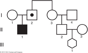So the probability that III-1 inherits the CF allele from II-2 is , or 1/8. We now extend the calculation to determine the probability that III-1 could inherit the cystic fibrosis allele from his mother, II-3. Individual II-3 does not have CF, but we are not sure whether or not she is a carrier. If the frequency (q) of the disease allele in the population is 0.025, then the probability that an unaffected individual such as II-3 is a carrier is 2pq/(1 − q²) = 0.049. If II-3 is a carrier, then there is a chance she will transmit the disease allele to III-1. These are all independent probabilities, so we can use the product rule. The probability that III-1 will have cystic fibrosis is

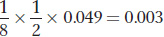
The frequency of cystic fibrosis among Caucasians is p² = (0.025)² = 0.000625. These calculations tell us that individuals who have a first cousin with cystic fibrosis have a 0.003 ÷ 0.000625 = 4.9-fold higher risk of having a child with the disease than members of the general population.

Here is another application of population genetics to assessing disease risk. Sickle-cell anemia, a recessive disease, has a frequency of about 0.25 percent, or 1 in 400, among African Americans (see Chapter 6). Applying the Hardy–Weinberg law, we estimate the frequency of the disease allele (Hb^S) as 0.05. What would be the expected frequency of this disease among the offspring of African Americans who are first cousins? Using the method described in Box 18-2, we calculate that the inbreeding coefficient (F) for the offspring of first-cousin marriages is 1/16. In the section on inbreeding above, we saw that the frequency of the homozygotes when there is inbreeding is increased, as shown by this equation:

Using this equation, we obtain

This represents a 2.2-fold increase in the risk of having a child with the disease for first-cousin marriages compared to that in a marriage between unrelated individuals.

Criminals can leave DNA evidence at the scene of a crime in the form of blood, semen, hairs, or even buccal cells from saliva on a cigarette butt. The polymerase chain reaction (PCR) enables forensic scientists to amplify very tiny amounts of DNA and determine the genotype of the individual who left the specimen. If the DNA found at the crime scene matches that of the suspect, then they “may be” the same individual. The key phrase here is “may be,” and this is where population genetics comes into play. Let’s see how this works.

Consider two microsatellite loci, each with multiple alleles: A₁, A₂, … A_n and B₁, B₂, … B_n. Forensic scientists determine that a DNA specimen from a crime scene and the suspect are both A₃/A₈ B₁/B₇. They have determined that there is a “match” between the evidence and the suspect. Does the match prove that the DNA evidence came from the suspect? Does it prove that that the suspect was at the crime scene?

What population geneticists do with this type of evidence is to test a specific hypothesis: The evidence came from someone other than the suspect. This is what statisticians call the “null hypothesis,” or the hypothesis that is considered true unless the evidence shows that it is very unlikely (see Chapter 4). To perform the test, we calculate the probability of observing a match between the evidence and the suspect, given that the suspect and the person who left the evidence are different individuals. Symbolically, we write

where “|” means “given.” If this probability is very small, then we can reject the null hypothesis and argue in favor of an alternative hypothesis: The evidence was left by the suspect. We never formally prove the suspect left the evidence since there could be alternative hypotheses such as The evidence was left by the suspect’s identical twin.

To calculate the probability of observing a match between the evidence and the suspect if the evidence is from a different individual, we need to know the frequencies of the microsatellite alleles in the population.

Prob(match | different individuals) is the same as the probability that the evidence came from a randomly chosen individual. We can calculate this probability using the allele frequencies above. First, we will assume that the Hardy–Weinberg law applies and calculate the probability of being A₄/A₆ at the first locus and B₁/B₇ at the second:

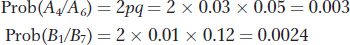
To combine these two probabilities, we need to make one more assumption. We need to assume that the two loci are independent; that is, that the loci are at linkage equilibrium. By making this assumption, we can apply the product rule for independent events (see Chapter 2) and determine that

Thus, the probability under the null hypothesis that the evidence came from someone other than the suspect is 7.2 × 10⁻⁶, or about 7 in a million. That’s a small probability, and so the null hypothesis seems unlikely in this case. However, if Prob(match | different individuals) were 0.1, then 10 percent of the population would be a match and could have left the evidence. In that case, we would not want to reject the null hypothesis.

Two microsatellites do not provide very much power to discriminate, so the FBI in the United States uses a set of 13 microsatellites. Microsatellite loci typically have large numbers of alleles (10 to 20 or more); therefore, the number of possible genotypes based on 13 microsatellites is astronomically large. With 10 alleles per locus, there are 55 possible genotypes at each locus and 55¹³, or 4.2 × 10²², possible multilocus genotypes for 13 loci. The FBI has also assembled a database called CODIS (Combined DNA Index System) that contains the frequencies of different alleles at these loci in the population, including data specific to different ethnic groups and regions of the country.

In this chapter, we have reviewed the basic principles of population genetics and discussed many applications to human genetics. Basic population genetic theory has been around for nearly 100 years, but only in the last decade has the development of high-throughput DNA-based technologies for genotyping individuals brought the complex patterns of variation among and within human populations into sharp focus. Not only has it been possible to unravel many of the details about how and when humans populated the globe from our African homeland, but geneticists have gained a deep understanding of how forces such as natural selection and genetic drift have shaped who we are.

What does the future hold? Soon, the sequencing of a human genome may cost little more than a new bicycle. A college student might swab the inside of her mouth with a Q-tip and deposit the sample in a kiosk while out to hear a band. Weeks later, she would be able to view her genome sequence on a Web site, compare it to those of her friends and relatives, and learn about her ancestry. As we’ll see in the next chapter, our ability to predict a person’s disease risks, talents, and other traits from his or her genotype is improving. To the extent that someone’s taste in music or love of extreme sports has genetic underpinnings, a person could in theory “Google” DNA mates likely to share similar interests. The DNA technology and population genetics theory are already in place; however, there are social and ethical questions to be addressed. Can and how will the information be kept private? Are there any limits on what a person should know about his or her own sequence? Should the government sequence everyone’s genome when he or she is born? Could medical insurance providers require that their clients submit their genome sequences? An understanding of the science can aid in determining how these questions are answered.