Chapter 13: Two-Way Analysis of Variance

13.1 13.1 The Two-Way ANOVA Model

698

When you complete this section, you will be able to:

• Discuss the advantages of a two-way ANOVA design.
• Describe the two-way ANOVA model and when it is used for inference.
• Interpret the relationship between two factors in terms of main effects and interaction.
• Construct an interaction plot and determine whether it shows that there is interaction among the factors.

We begin with a discussion of the advantages of the two-way ANOVA design, illustrated through some examples. Then we discuss the model.

Advantages of two-way ANOVA

In one-way ANOVA, we classify populations according to one categorical variable, or factor. In the two-way ANOVA model, there are two factors, each with its own number of levels. When we are interested in the effects of two factors, a two-way design offers great advantages over several single-factor studies.

factor, p. 644

EXAMPLE 13.1

Design 1: Does haptic feedback improve performance? In Example 12.1 (page 645), a group of technology students wanted to see if haptic feedback is helpful in navigating a simulated game environment. To do this, they plan to randomly assign 20 students to each of three joystick controller types and record the time it takes to complete a navigation mission.

It turns out that their simulated game has four difficulty levels. Suppose that a second experiment is planned to compare these levels when using the standard joystick. A similar experimental design will be used, with the four difficulty levels randomly assigned equally among the 60 students.

Here is a picture of the designs of the first and second experiments with the sample sizes:

Joystick	n
1	20
2	20
3	20
Total	60

Difficulty	n
1	15
2	15
3	15
4	15
Total	60

699

In the first experiment, 20 students were assigned to each level of the factor for a total of 60 students. In the second experiment, 15 students were assigned to each level of the factor for a total of 60 students. If each experiment takes one week, the total amount of time for the two experiments is two weeks.

Each experiment will be analyzed using one-way ANOVA. The factor in the first experiment is joystick type with three levels, and the factor in the second experiment is game difficulty with four levels. Let’s now consider combining the two experiments into one.

EXAMPLE 13.2

Design 2: Does haptic feedback improve performance regardless of difficulty level? Suppose that we use a two-way approach for the simulated game problem. There are two factors, joystick type and difficulty. Because joystick type has three levels and difficulty has four levels, this is a 3 × 4 design. This gives a total of 12 possible combinations of type and difficulty. With a total of 60 students, we could assign each combination of type and difficulty to five students. The time it takes to complete a navigation mission is the outcome variable.

Here is a picture of the two-way design with the sample sizes:

	Difficulty
Joystick	1	2	3	4	Total
1	5	5	5	5	20
2	5	5	5	5	20
3	5	5	5	5	20
Total	15	15	15	15	60

Each combination of the factors in a two-way design corresponds to a cellcell. The 3 × 4 ANOVA for the haptic feedback experiment has 12 cells, each corresponding to a particular combination of joystick type and difficulty level.

With the two-way design, notice that we have 20 students assigned to each joystick type, the same as we had for the one-way experiment for type alone. Similarly, there are still 15 students assigned to each level of difficulty. Thus, the two-way design gives us the same amount of information for estimating the completion time for each level of each factor as we had with the two one-way designs. The difference is that we can collect all the information in only one experiment. This experiment lasts one week (instead of a combined two weeks) and involves a single observation from each of the 60 students. By combining the two factors into one experiment, we have increased our efficiency by reducing the amount of data to be collected by half.

EXAMPLE 13.3

The effect of a limited time offer on purchase intent. Starbucks’ Pumpkin Spice Latte (PSL) is the company’s most popular seasonal item. Why is this? Is it the unique flavor? Or could it be because it is only available for a limited time each year? To investigate this, some students surveyed 100 Starbucks consumers about their intent to purchase a PSL when it is offered in the fall.¹ Half of the surveys included the upcoming PSL advertisement. The other half included the same advertisement with the additional words “Limited Time Offer’’ above the image of the drink. Because purchase intent may depend on how frequently a consumer visits Starbucks, the students included a survey question about this. The question was used to classify each customer as either a “light’’ or “heavy’’ user of Starbucks.

700

The factors for the two-way ANOVA are advertisement type with two levels and user status with two levels. There are 2 × 2 = 4 cells in their study. The outcome variable purchase intent is measured on a 1 to 7 scale.

Here is a table of sample sizes that summarizes their design:

	User status
Advertisement	Light	Heavy	Total
Regular	27	23	50
Added wording	19	31	50
Total	46	54	100

The students were not able to control the number of subjects in each cell of the study because they did not know user status until the survey was administered.

This example illustrates another advantage of two-way designs. Although the students are primarily interested in the effect of adding the words “Limited Time Offer’’ on purchase intent, they also included user status because they suspected that the wording effect might be different in light and heavy users.

Consider an alternative one-way design where we ignore user status. With this design, we will have the same number of customers at each of the ad type levels, so in this way, it is similar to our two-way design.

However, suppose that there are, in fact, differences due to user status. In this case, the one-way ANOVA would assign this variation to the RESIDUAL (within groups) part of the model. In the two-way ANOVA, user status is included as a factor; therefore, this variation is included in the FIT part of the model. Whenever we can move variation from RESIDUAL to FIT, we reduce the σ of our model and increase the power of our tests.

DATA = FIT + RESIDUAL, p. 560

EXAMPLE 13.4

Professor Pietro M. Motta / Science Source

Vitamin D and osteoporosis. Osteoporosis is a disease primarily of the elderly. People with osteoporosis have low bone mass and an increased risk of bone fractures. More than 10 million people in the United States, 1.4 million Canadians, and many millions throughout the world have this disease. Adequate calcium in the diet is necessary for strong bones, but vitamin D is also needed for the body to efficiently use calcium. High doses of calcium in the diet will not prevent osteoporosis unless there is adequate vitamin D. Exposure of the skin to the ultraviolet rays in sunlight enables our bodies to make vitamin D. However, elderly people often don’t go outside as much as younger people do, and in northern areas such as Canada, there is not sufficient ultraviolet light for the body to make vitamin D, particularly in the winter months.

701

Suppose that we wanted to see if calcium supplements will increase bone mass (or prevent a decrease in bone mass) in an elderly Canadian population. Because of the vitamin D complication, we will make this a factor in our design. We will use a 2 × 2 design for our osteoporosis study. The two factors are calcium and vitamin D. The levels of each factor will be zero (placebo) and an amount that is expected to be adequate, 800 milligrams per day (mg/d) for calcium and 300 international units per day (IU/d) for vitamin D.

Women between the ages of 70 and 80 will be recruited as subjects. Bone mineral density (BMD) will be measured at the beginning of the study, and supplements will be taken for one year. The change in BMD over the one-year period is the outcome variable. We expect a dropout rate of 20%, and we would like to have about 20 subjects providing data in each group at the end of the study. We will, therefore, recruit 100 subjects and randomly assign 25 to each treatment combination.

Here is a table that summarizes the design with the sample sizes at the start of the study:

	Vitamin D
Calcium	Placebo	300 IU/d	Total
Placebo	25	25	50
800 mg/d	25	25	50
Total	50	50	100

This example illustrates a third reason for using two-way designs. The effectiveness of the calcium supplement on BMD may differ across the two levels of vitamin D. We call this an interactioninteraction. In contrast, the average values for the calcium effect and the vitamin D effect are represented as main effectsmain effects. The two-way model represents FIT as the sum of a main effect for each of the two factors and an interaction. One-way designs that vary a single factor and hold other factors fixed cannot discover interactions. We will discuss interactions more fully later.

These examples illustrate several reasons two-way designs are preferable to one-way designs.

ADVANTAGES OF TWO-WAY ANOVA

1. It is more efficient to study two factors simultaneously rather than separately.
2. We can reduce the residual variation in a model by including a second factor thought to influence the response.
3. We can investigate interactions between factors.

702

These considerations also apply to study designs with more than two factors. We will be content, however, to explore only the two-way case in this chapter. Remember that the choice of sampling or experimental design is fundamental to any statistical study. Factors and levels must be carefully selected by an individual or team who understands both the statistical models and the issues that the study will address.

The two-way ANOVA model

When discussing two-way models in general, we will use the labels A and B for the two factors. For particular examples and when using statistical software, it is better to use meaningful names for these categorical variables. Thus, in Example 13.2 (page 699), we would say that the factors are joystick type and difficulty level, and in Example 13.4, we would say that the factors are the calcium and vitamin D.

The numbers of levels of the factors are often used to describe the model. Again using our earlier examples, we would say that Example 13.2 represents a 3 × 4 ANOVA, and Example 13.4 illustrates a 2 × 2 ANOVA. In general, Factor A will have I levels, and Factor B will have J levels. Therefore, we call the general two-way problem an I × J ANOVA.

In a two-way design, every level of A appears in combination with every level of B, so that I × J groups are compared. The sample size for level i of Factor A and level j of Factor B is . In Examples 13.2 and 13.4 the have been equal but this is not required.² The total number of observations is

ASSUMPTIONS FOR TWO-WAY ANOVA

We have independent simple random samples (SRSs) of size from each of I × J Normal populations. The population means may differ, but all populations have the same standard deviation σ. The and σ are unknown parameters.

Let represent the kth observation from the population having Factor A at level i and Factor B at level j. The statistical model is

for i = 1, . . . , I and j = 1, . . . , J and , where the deviations are from an N(0, σ) distribution.

estimates of population parameters p. 653

Similar to the one-way model, the FIT part is the group means , and the RESIDUAL part is the deviations of the individual observations from their group means. To estimate a group mean , we use the sample mean of the observations in the samples from this group:

703

The k below the means that we sum the observations that belong to the (i, j)th sample.

The RESIDUAL part of the model contains the unknown σ. We first calculate the sample variances for each SRS. Provided it is reasonable to consider a common standard deviation (page 654), we pool these to estimate σ²:

Just as in one-way ANOVA, the numerator in this fraction is SSE and the denominator is DFE. Also, DFE is the total number of observations minus the number of groups. That is, . The estimator of σ is s_p.

USE YOUR KNOWLEDGE

Question 13.1

13.1 Limited-time offer effect on purchase intent. Example 13.3 (page 699) describes a study designed to compare different advertisement types and user status on purchase intent. Write out the ANOVA model for this study. Be sure to give specific values for I, J, and the . List all the parameters of the model.

Question 13.2

13.2 Limited-time offer effect on purchase intent, continued. Refer to the previous exercise. The following table summarizes the group means and standard deviations.

	Light user		Heavy user
Advertisement		s		s
Regular	4.56	1.75	5.00	1.79
Added wording	5.74	1.19	5.19	1.91

(a) Is it reasonable to pool the standard deviations for these data? Explain your answer.
(b) For each parameter in your model from Exercise 13.1, give the estimate.

Main effects and interactions

In this section, we will further explore the FIT part of the two-way ANOVA, which is represented in the model by the population means . The two-way design gives some structure to the set of means .

So far, because we have independent samples from each of I × J groups, we have presented the problem as a one-way ANOVA with groups. Each population mean is estimated by the corresponding sample mean and we can calculate sums of squares and degrees of freedom as in one-way ANOVA. In accordance with the conventions used by many computer software packages, we use the term model when discussing the sums of squares and degrees of freedom calculated as in one-way ANOVA with groups. Thus, SSM is a model sum of squares constructed from deviations of the form , where is the average of all the observations and is the mean of the (i, j)th group. Similarly, DFM is simply .

704

In two-way ANOVA, the terms SSM and DFM can be further broken down into terms corresponding to a main effect for A, a main effect for B, and an AB interaction. Each of SSM and DFM is then a sum of terms:

SSM = SSA + SSB + SSAB

and

DFM = DFA + DFB + DFAB

The term SSA represents variation among the means for the different levels of Factor A. Because there are I such means, DFA = I − 1 degrees of freedom. Similarly, SSB represents variation among the means for the different levels of Factor B, with DFB = J − 1.

Interactions are a bit more involved. We can see that SSAB, which is SSM − SSA − SSB, represents the variation in the model that is not accounted for by the main effects. By subtraction we see that its degrees of freedom are

There are many kinds of interactions. The easiest way to study them is through examples.

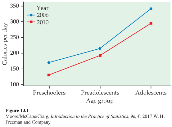
EXAMPLE 13.5

Investigating differences in sugar-sweetened beverage consumption. Consumption of sugar-sweetened beverages has been linked to Type 2 diabetes and obesity. One study used data from the National Health and Nutrition Examination Survey (NHANES) to estimate consumption of these beverages among children. More than 14,000 individuals provided data for this study. Individuals were divided into three age categories: preschoolers (two to five years old), preadolescents (6 to 11 years old), and adolescents (12 to 19 years old).³ Here are the means for the number of calories in sugar-sweetened beverages consumed per day during 2003 to 2006 and 2007 to 2010:

	Year
Group	2006	2010	Mean
Preschoolers	170	130	150
Preadolescents	214	192	203
Adolescents	341	295	318
Mean	242	206	224

The table in Example 13.5 includes averages of the means in the rows and columns. For example, in 2006 the mean of calories consumed per day is

which is rounded to 242 in the table. Similarly, the corresponding value for 2010 is

705

which is rounded to 206 in the table. These averages are called marginal meansmarginal means (because of their location at the margins of such tabulations). The grand mean (224 in this case) can be obtained by averaging either set of marginal means.

Figure 13.1 is a plot of the group means. From the plot, we see that fewer calories from sugar-sweetened beverages were consumed by each group in 2010 than in 2006. In statistical language, there is a main effect for year. We also see that the means are different across age categories. This means there is a main effect for age. These main effects can be described by differences between the marginal means. For example, the mean for 2006 is 242 calories and decreases 36 calories to 206 calories in 2010. Similarly, the mean for preschoolers is 150, it increases 53 calories to 203 for preadolescents, and then increases 115 calories to 318 for adolescents.

To examine two-way ANOVA data for a possible interaction, always construct a plot similar to Figure 13.1. When no interaction is present, the marginal means provide a reasonable description of the two-way table of means. This will be reflected in the plot by profiles that are roughly parallel. In this case, it is debatable whether the two profiles (the collections of marginal means for a given year) should be considered parallel.

When there is an interaction, the marginal means do not tell the whole story. For example, with these data, the marginal mean difference between years is 36 calories. This is smaller than the difference in calories for the preschoolers (170 − 130 = 40) and adolescents (341 − 295 = 46) and larger than the change in the preadolescents (214 − 192 = 22). If differences of roughly 20 calories per day are scientifically meaningful, then we would say that it appears there is an interaction. Inference is still needed to confirm that these differences are not likely the result of chance variation.

Figure 13.1: FIGURE 13.1 Plot of the mean calories in sugar-sweetened beverages consumed per day in 2003 to 2006 and 2007 to 2010 for different age groups, Example 13.5.

706

Interactions come in many shapes and forms. When we find an interaction, a careful examination of the means is needed to properly interpret the data. Simply stating that interactions are significant tells us very little. Plots of the group means, called interaction plotsinteraction plots, are essential. Here is another example.

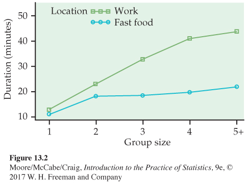
EXAMPLE 13.6

Eating in groups. Some research has shown that people eat more when they eat in groups. One possible mechanism for this phenomenon is that they may spend more time eating when in a larger group. A study designed to examine this idea measured the length of time spent (in minutes) eating lunch in different settings.⁴ Here are some data from this study:

	Number of people eating
Lunch setting	1	2	3	4	5 or more	Mean
Workplace	12.6	23.0	33.0	41.1	44.0	30.7
Fast-food restaurant	10.7	18.2	18.4	19.7	21.9	17.8
Mean	11.6	20.6	25.7	30.4	32.9	24.2

Figure 13.2 gives the plot of the means for this example. The patterns are not parallel, so it appears that we have an interaction. Meals take longer when there are more people present, but this phenomenon is much greater for the meals consumed at work. For fast-food eating, the meal durations are fairly similar when there is more than one person present.

Figure 13.2: FIGURE 13.2 Plot of mean meal duration versus lunch setting and group size, Example 13.6.

A different kind of interaction is present in the next example. Here, we must be very cautious in our interpretation of the main effects because either one of them can lead to a distorted conclusion.

EXAMPLE 13.7

We got the beat? When we hear music that is familiar to us, we can quickly pick up the beat, and our mind synchronizes with the music. However, if the music is unfamiliar, it takes us longer to synchronize. In a study that investigated the theoretical framework for this phenomenon, French and Tunisian nationals listened to French and Tunisian music.⁵ Each subject was asked to tap in time with the music being played. A synchronization score, recorded in milliseconds, measured how well the subjects synchronized with the music. A higher score indicates better synchronization. Six songs of each music type were used. Here are the means:

707

	Music
Nationality	French	Tunisian	Mean
French	950	750	850
Tunisian	760	1090	925
Mean	855	920	887

The means are plotted in Figure 13.3. In the study, the researchers were not interested in main effects. Their theory predicted the interaction that we see in the figure. Subjects synchronize better with music from their own culture. The main effects, on the other hand, suggest that Tunisians sychronize better than the French (regardless of music type) and that it is easier to synchronize to Tunisian music (regardless of nationality).

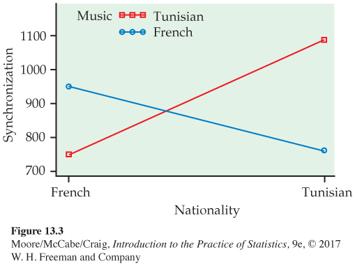
Figure 13.3: FIGURE 13.3 Plot of mean synchronization score versus type of music for French and Tunisian nationals, Example 13.7.

The interaction in Figure 13.3 is very different from those that we saw in Figure 13.1 and 13.2. These examples illustrate the point that it is necessary to plot the means and carefully describe the patterns when interpreting an interaction.

The design of the study in Example 13.7 allows us to examine two main effects and an interaction. However, this setting does not meet all the assumptions needed for statistical inference using the two-way ANOVA framework of this chapter. As with one-way ANOVA, we require that observations be independent.

In this study, we have a design that has each subject contributing data for two types of music, so these two scores will be dependent. The framework is similar to the matched pairs setting (page 182). The design is called a repeated-measures designrepeated-measures design. More advanced texts on statistical methods cover this important design.

708

USE YOUR KNOWLEDGE

Question 13.3

13.3 What’s wrong? In each of the following, identify what is wrong and then either explain why it is wrong or change the wording of the statement to make it true.

(a) A two-way ANOVA is used when the outcome variable can take only two possible values.
(b) In a 2 × 3 ANOVA, each level of Factor A appears with two levels of Factor B.
(c) The FIT part of the model in a two-way ANOVA represents the variation that is sometimes called error or residual.
(d) In an

Question 13.4

13.4 What’s wrong? In each of the following, identify what is wrong and then either explain why it is wrong or change the wording of the statement to make it true.

(a) Parallel profiles of cell means imply that a strong interaction is present.
(b) You can perform a two-way ANOVA only when the sample sizes are the same in all cells.
(c) The estimate is obtained by pooling the marginal sample variances.
(d) When interaction is present, the marginal means are always uninformative.