As we move about from place to place, we encounter objects in specific locations. If we had no awareness of location, the world would be a bewildering mass of visual information. The next leg of our journey down the neural roads traces how the brain constructs a spatial map. In Clinical Focus 9-1, the photograph has a left and a right, an up and a down. All these elements must be coded separately in the brain.

Neural coding of location begins in the retina and is maintained throughout all visual pathways. To understand how this spatial coding is accomplished, imagine your visual world as seen by your two eyes. Imagine the large red and blue rectangles in Figure 9-20 as a wall. Focus your gaze on the black cross in the middle of the wall.

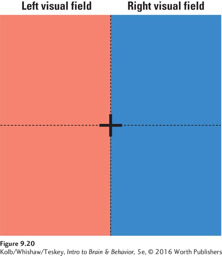
The part of the wall that you can see without moving your head is your visual field. It can be divided into two halves, the left and right visual fields, by drawing a vertical line through the middle of the black cross. Now recall from Figure 9-10 that the left half of each retina looks at the right side of the visual field, whereas the right half of each retina looks at the visual field’s left side. Thus, input from the right visual field goes to the left hemisphere, and input from the left visual field goes to the right hemisphere.

Therefore, the brain can easily determine whether visual information lies to the left or right of center. If input goes to the left hemisphere, the source must be in the right visual field; if input goes to the right hemisphere, the source must be in the left visual field. This arrangement tells you nothing about the precise location of an object in the left or right side of the visual field, however. To understand how precise spatial localization is accomplished, we must return to the retinal ganglion cells.

302

Look again at Figure 9-8 and you can see that each RGC receives input through bipolar cells from several photoreceptors. In the 1950s, Stephen Kuffler, a pioneer in visual system physiology, made an important discovery about how photoreceptors and retinal ganglion cells are linked (Kuffler, 1952). By shining small spots of light on the receptors, he found that each ganglion cell responds to stimulation on just a small circular patch of the retina—the ganglion cell’s receptive field.

A ganglion cell’s receptive field is therefore the retinal region on which it is possible to influence that cell’s firing. Stated differently, the receptive field represents the outer world as seen by a single cell. Each RGC sees only a small bit of the world, much as you would if you looked through a narrow cardboard tube. The visual field is composed of thousands of such receptive fields (illustrated on page 286).

Now let us consider how receptive fields enable the visual system to interpret an object’s location. Imagine that the retina is flattened like a piece of paper. When a tiny light shines on different parts of the retina, different ganglion cells respond. For example, when a light shines on the top left corner of the flattened retina, a particular RGC responds because that light is in its receptive field. Similarly, when a light shines on the top right corner, a different RGC responds.

By using this information, we determine the location of a light on the retina by the ganglion cell it activates. Another location device is determining where the light must come from to hit a particular place on the retina. Light coming from above hits the bottom of the retina after passing through the eye’s lens, and light from below hits the top of the retina. Information at the top of the visual field stimulates ganglion cells on the bottom of the retina; information at the bottom of the field stimulates ganglion cells on the top of the retina.

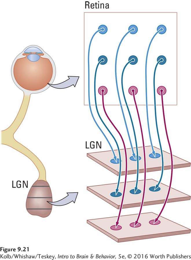
Now consider the connection from the ganglion cells to the lateral geniculate nucleus. In contrast to the retina, the LGN is not a thin sheet; it is shaped more like a sausage. We can compare it to a stack of sausage slices, with each slice representing a layer of cells.

Figure 9-21 shows how the connections from the retina to the LGN can represent location. A retinal ganglion cell that responds to light in the top left region of the retina connects to the left side of the first card. A retinal ganglion cell that responds to light in the bottom right region of the retina connects to the right side of the last card. In this way, the location of left–right and top–bottom information is maintained in the LGN.

Like the ganglion cells, each LGN cell has a receptive field—the region of the retina that influences its activity. If two adjacent retinal ganglion cells synapse on a single LGN cell, the receptive field of that LGN cell will be the sum of the two ganglion cells’ receptive fields. As a result, the receptive fields of LGN cells are bigger than those of RGCs.

The LGN projection to the striate cortex (region V1) also maintains spatial information. As each LGN cell, representing a particular place, projects to region V1, a spatially organized neural representation—a topographic map—is produced in the cortex. As illustrated in Figure 9-22, this representation is essentially a map of the visual world.

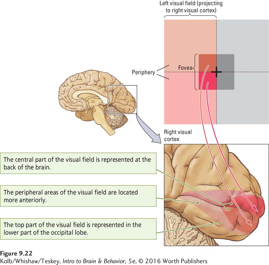
The central part of the visual field is represented at the back of the brain, whereas the periphery is represented more anteriorly. The upper part of the visual field is represented at the bottom of region V1 and the lower part at the top of V1. The other regions of the visual cortex (such as V3, V4, and V5) have topographical maps similar to that of V1. Thus the V1 neurons must project to the other regions in an orderly manner, just as the LGN neurons project to region V1 in an orderly way.

303

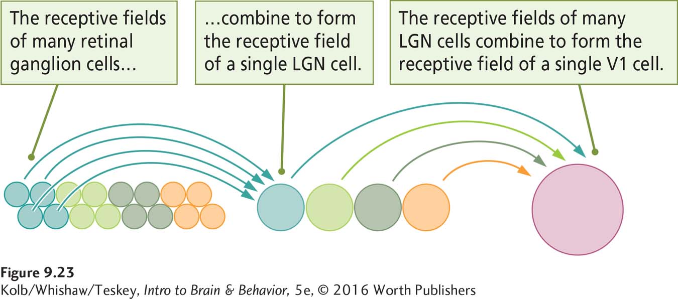
Within each visual cortical area, each neuron’s receptive field corresponds to the part of the retina to which the neuron is connected. As a rule of thumb, cells in the cortex have much larger receptive fields than RGCs do. This large field size means that the receptive field of a cortical neuron must be composed of the receptive fields of many RGCs, as illustrated in Figure 9-23.

One additional wrinkle pertains to the organization of topographic maps. Harry Jerison (1973) proposed the principle of proper mass, which states that the amount of neural tissue responsible for a particular function is proportional to the amount of neural processing that function requires. The more complex a function is, the larger a specific region performing that function must be. The visual cortex provides some good examples.

You can see in Figure 9-3). In other words, sensory areas that have more cortical representation provide a more detailed construct of the external world.

304

Topographic mapping based on neuronal receptive fields is an effective way for the brain to code object location. But if the left visual field is represented in the right cerebral hemisphere and the right visual field is represented in the left cerebral hemisphere, how are the two halves of the visual field ultimately merged into a unified representation? After all, we have the subjective impression not of two independent visual fields but rather of a single, continuous field of vision.

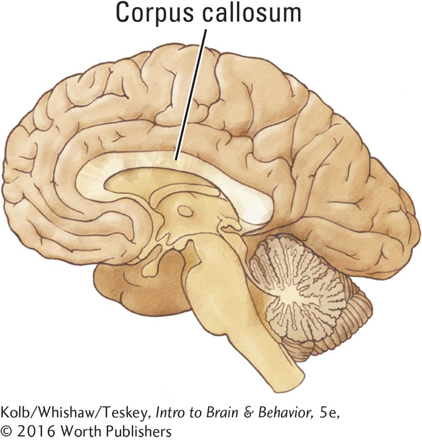
The answer to how this unity is accomplished lies in the corpus callosum, which binds the two sides of the visual field together at the midline. Until the 1950s, its function was largely a mystery. Physicians had occasionally cut the corpus callosum to control severe epilepsy or to reach a very deep tumor, but patients did not appear much affected by this surgery. The corpus callosum clearly linked the two hemispheres of the brain, but exactly which parts were connected was not yet known.

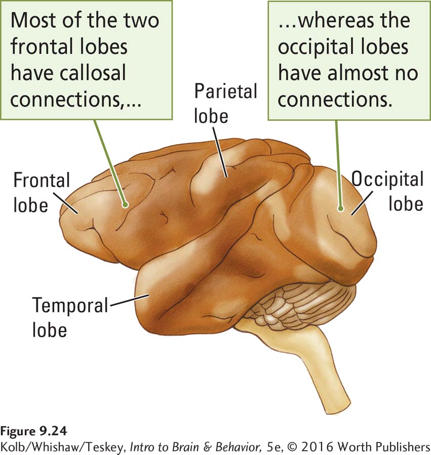
We now realize that the corpus callosum connects only certain brain structures. As shown in Figure 9-24, the frontal lobes have many callosal connections, but the occipital lobes have almost none. If you think about it, there is no reason for a neuron in the visual cortex that is looking at one place in the visual field to be concerned with what another neuron in the opposite hemisphere is looking at in another part of the visual field.

Cells that lie along the midline of the visual field are an exception, however. These cells look at adjacent places in the visual field, one slightly to the left of center and one slightly to the right. Callosal connections between such cells zip the two visual fields together by combining their receptive fields to overlap at the midline. The two fields thus become one.

Location in the Visual World

Before you continue, check your understanding.

Question 1

Question 2

Question 3

Question 4

Question 5

Answers appear in the Self Test section of the book.