Reconciling the Two Interest Rate Models
In Module 28 we developed what is known as the liquidity preference model of the interest rate. In that model, the equilibrium interest rate is the rate at which the quantity of money demanded equals the quantity of money supplied in the money market. In the loanable funds model, we see that the interest rate matches the quantity of loanable funds supplied by savers with the quantity of loanable funds demanded for investment spending. How do the two models compare?
The Interest Rate in the Short Run
As we explained using the liquidity preference model, a fall in the interest rate leads to a rise in investment spending, I, which then leads to a rise in both real GDP and consumer spending, C. The rise in real GDP doesn’t lead only to a rise in consumer spending, however. It also leads to a rise in savings: at each stage of the multiplier process, part of the increase in disposable income is saved. How much do savings rise? According to the savings–
Figure 29.7 shows how our two models of the interest rate are reconciled in the short run by the links among changes in the interest rate, changes in real GDP, and changes in savings. Panel (a) represents the liquidity preference model of the interest rate. MS1 and MD1 are the initial supply and demand curves for money. According to the liquidity preference model, the equilibrium interest rate in the economy is the rate at which the quantity of money supplied is equal to the quantity of money demanded in the money market. Panel (b) represents the loanable funds model of the interest rate. S1 is the initial supply curve and D is the demand curve for loanable funds. According to the loanable funds model, the equilibrium interest rate in the economy is the rate at which the quantity of loanable funds supplied is equal to the quantity of loanable funds demanded in the market for loanable funds.
| Figure 29.7 | The Short- |
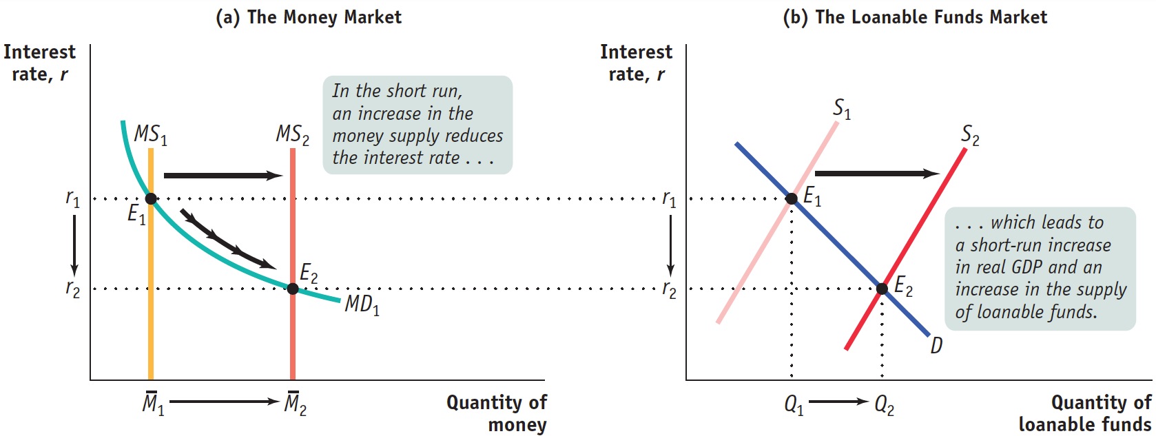
 1 to 2, pushes the equilibrium interest rate down, from r1 to r2. Panel (b) shows the loanable funds model of the interest rate. The fall in the interest rate in the money market leads, through the multiplier effect, to an increase in real GDP and savings; to a rightward shift of the supply curve of loanable funds, from S1 to S2; and to a fall in the interest rate, from r1 to r2. As a result, the new equilibrium interest rate in the loanable funds market matches the new equilibrium interest rate in the money market at r2.
In Figure 29.7 both the money market and the market for loanable funds are initially in equilibrium at E1 with the same interest rate, r1. You might think that this would happen only by accident, but in fact it will always be true. To see why, let’s look at what happens when the Fed increases the money supply from 1 to 2. This pushes the money supply curve rightward to MS2, causing the equilibrium interest rate in the market for money to fall to r2, and the economy moves to a short-
In the short run, then, the supply and demand for money determine the interest rate, and the loanable funds market follows the lead of the money market. When a change in the supply of money leads to a change in the interest rate, the resulting change in real GDP causes the supply of loanable funds to change as well. As a result, the equilibrium interest rate in the loanable funds market is the same as the equilibrium interest rate in the money market.
Notice our use of the phrase “in the short run.” Changes in aggregate demand affect aggregate output only in the short run. In the long run, aggregate output is equal to potential output. So our story about how a fall in the interest rate leads to a rise in aggregate output, which leads to a rise in savings, applies only to the short run. In the long run, as we’ll see next, the determination of the interest rate is quite different because the roles of the two markets are reversed. In the long run, the loanable funds market determines the equilibrium interest rate, and it is the market for money that follows the lead of the loanable funds market.
The Interest Rate in the Long Run
AP® Exam Tip
To determine which graph to draw for an AP® exam question, watch for mentions of the money market, which indicate that you should draw a money market graph with a vertical supply curve, or mentions of loanable funds, which suggest that you should draw a loanable funds market graph with an upward-
In the short run an increase in the money supply leads to a fall in the interest rate, and a decrease in the money supply leads to a rise in the interest rate. In the long run, however, changes in the money supply don’t affect the interest rate.
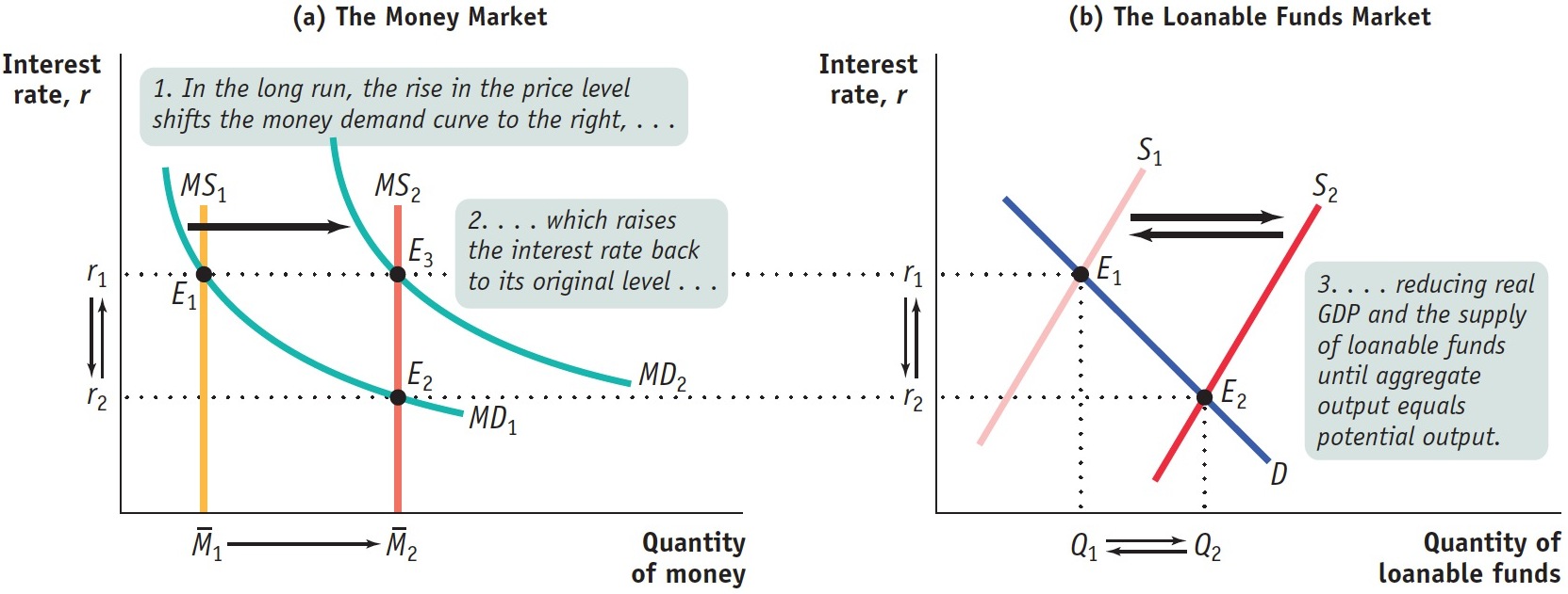
Figure 29.8 shows why. As in Figure 29.7, panel (a) shows the liquidity preference model of the interest rate and panel (b) shows the supply and demand for loanable funds. We assume that in both panels the economy is initially at E1, in long-1. The demand curve for loanable funds is D, and the initial supply curve for loanable funds is S1. The initial equilibrium interest rate in both markets is r1.
| Figure 29.8 | The Long- |
 1 to 2; panel (b) shows the corresponding long-
Now suppose the money supply rises from 1 to 2. As we saw in Figure 29.7, this initially reduces the interest rate to r2. However, in the long run the aggregate price level will rise by the same proportion as the increase in the money supply (due to the neutrality of money, a topic presented in detail in the next section). A rise in the aggregate price level increases money demand by the same proportion. So in the long run the money demand curve shifts out to MD2, and the equilibrium interest rate rises back to its original level, r1.
Panel (b) of Figure 29.8 shows what happens in the market for loanable funds. We saw earlier that an increase in the money supply leads to a short-
In the long run, then, changes in the money supply do not affect the interest rate. So what determines the interest rate in the long run—