9.2 The Sources of Long-Run Growth
Long-
The Crucial Importance of Productivity
Labour productivity, often referred to as Average Productivity of Labour (APL) or simply productivity, is (real) output per worker or, in some cases, output per hour.
Sustained economic growth occurs only when the amount of output produced by the average worker increases steadily. The terms labour productivity, or Average Productivity of Labour (APL) or simply productivity for short, are used to refer either to output per worker or, in some cases, to output per hour. (The number of hours worked by an average worker differs to some extent across countries, although this isn’t an important factor in the difference between living standards in, say, India and Canada.) In this book we’ll focus on output per worker. For the economy as a whole, productivity—
You might wonder why we say that higher productivity is the only source of long-
Over the longer run, however, the rate of employment growth is never very different from the rate of population growth. Over the course of the twentieth century, for example, Canada’s population rose at an average rate of about 1.7% per year and employment rose by 2.1% per year. Real GDP per capita rose 2.0% per year; of that, 1.6%—that is, about 80% of the total—
So increased productivity is the key to long-
Explaining Growth in Productivity
There are three main reasons why the average Canadian worker today produces far more than his or her counterpart a century ago. First, on average, each modern worker has far more physical capital, such as machinery and office space, to work with. Second, the modern worker is much better educated and so possesses much more human capital. Finally, modern firms have the advantage of a century’s accumulation of technical advancements reflecting a great deal of technological progress.
Let’s look at each of these factors in turn.
Physical capital consists of human-
Increase in Physical Capital Economists define physical capital as manufactured resources such as buildings and machines. Physical capital makes workers more productive. For example, a farmworker operating a tractor can cultivate a lot more farmland per day than one equipped only with a shovel.
The average Canadian private-
Human capital is the improvement in labour created by the education and knowledge embodied in the workforce.
Increase in Human Capital It’s not enough for a worker to have good equipment—
Canada’s human capital has increased dramatically over the past century. A hundred years ago, most Canadians could read and write, but few had an extensive education. In 1920, only 3.2% of Canadians under the age of 25 were enrolled in university or college and about 3% of Canadians between 25 and 29 had a post-
Analyses based on growth accounting, described later in this chapter, suggest that education—
Technological progress is an advance in the technical means of the production of goods and services.
Technological Progress Probably the most important driver of productivity growth is technological progress, which is broadly defined as an advance in the technical means of the production of goods and services. We’ll see shortly how economists measure the impact of technology on growth.

Workers today are able to produce more than those in the past, even with the same amount of physical and human capital, because technology has advanced over time. It’s important to realize that economically important technological progress need not be flashy or rely on cutting-
Accounting for Growth: The Aggregate and Per Worker Production Functions
Aggregate real output for an economy is higher, other things equal, when i) more physical capital is used, ii) more labour (workers) is used, iii) more human capital is used, and/or iv) the technology improves. Economists use the aggregate production function to demonstrate this relation:

where
The aggregate production function is a relationship that shows how the aggregate real quantity of output is produced using the available factors of production (the inputs: labour, physical capital, and human capital) and technology [A and the function F(…)].
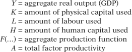
Total factor productivity — represented by the parameter A in the aggregate production function Y = A × F(K, L, H) helps account for output that is not a result of the productive inputs. That is, it captures all inputs and technological features left out of the aggregate production function.
This equation shows that if total factor productivity rises, then aggregate real output will also rise, all else the same4—a result that can be interpreted as an improvement in technology. We assume that a small increase in K, holding all other inputs and technology fixed, causes the amount of aggregate real output to rise by a marginal amount, called the positive marginal productivity of physical capital (positive MPK). We also assume that the marginal products of labour and human capital are both positive. If total factor productivity is held constant, then the production function F(…) shows how generous the technology is in increasing productivity, that is, how the technology magnifies the effect of inputs K, L, and H into aggregate real output. Similarly, if the levels of the inputs and the aggregate production remain fixed, then increases in total factor productivity can be interpreted as improvements in technology, since this allows for higher levels of real output to be produced without having to use more inputs.
The positive marginal productivity of physical capital (positive MPK) is the amount by which productivity is increased as the result of a small increase in physical capital used.
Likewise, productivity is higher, all else the same, when i) more physical capital is used, ii) human capital increases, and/or iii) the technology improves. In this case we assume that an increase in physical capital per worker causes a rise in real output per worker and that the same holds true for an increase in human capital per worker. So, when total factor productivity rises, then the real output per worker will rise. To quantify these effects, economists use the per worker production function, which shows how productivity depends on the quantities of physical capital per worker and human capital per worker as well as the state of technology:
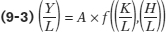
where
The per worker production function is a hypothetical function that shows how productivity (real GDP per worker) depends on the quantities of physical capital per worker and human capital per worker as well as the state of technology.
In general, all three factors on the right side of the function tend to rise over time, as workers, for example, are equipped with more machinery, receive more education, and benefit from technological advances. What the per worker production function does is allow economists to disentangle the effects of these three factors on overall productivity.
An example of a per worker production function applied to real data comes from a comparative study of Chinese and Indian economic growth by the economists Barry Bosworth and Susan Collins of the Brookings Institution. They used the following aggregate production function:

where A represents an estimate of the level of technology and they assumed that each year of education raises workers’ human capital by 7%. Using this function, they tried to explain why China grew faster than India between 1978 and 2004. About half the difference, they found, was due to China’s higher levels of investment spending, which raised its level of physical capital per worker faster than India’s. The other half was due to faster Chinese technological progress (growth in A).
A per worker production function exhibits diminishing returns to physical capital or diminishing marginal productivity of (physical) capital (dim MPK) when, holding the amount of human capital per worker and the state of technology fixed, each successive increase in the amount of physical capital per worker leads to a smaller increase in productivity.
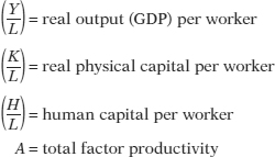
In analyzing historical economic growth, economists have discovered a crucial fact about the estimated per worker production function: it exhibits diminishing returns to physical capital. This is often called diminishing marginal productivity of (physical) capital (dimMPK). So when the amount of human capital per worker and the state of technology are held fixed, each successive increase in the amount of physical capital per worker leads to a smaller increase in productivity. The graph and table in Figure 9-4 give a hypothetical example of how the level of physical capital per worker might affect the level of real GDP per worker, holding human capital per worker and the state of technology fixed. In this example, we measure the quantity of physical capital in dollars.
To see why the relationship between physical capital per worker and productivity exhibits diminishing returns, think about how having farm equipment affects the productivity of farmworkers. A little bit of equipment makes a big difference: a worker equipped with a tractor can do much more than a worker without one. And a worker using more expensive equipment will, other things equal, be more productive: a worker with a $40 000 tractor will normally be able to cultivate more farmland in a given amount of time than a worker with a $20 000 tractor because the more expensive machine will be more powerful, perform more tasks, or both.
But will a worker with a $40 000 tractor, holding human capital and technology constant, be twice as productive as a worker with a $20 000 tractor? Probably not: there’s a huge difference between not having a tractor at all and having even an inexpensive tractor; there’s much less difference between having an inexpensive tractor and having a better tractor. And we can be sure that a worker with a $200 000 tractor won’t be 10 times as productive: a tractor can be improved only so much. Because the same is true of other kinds of equipment, the per worker production function shows diminishing returns to physical capital.
IT MAY BE DIMINISHED … BUT IT’S STILL POSITIVE
It’s important to understand what diminishing returns to physical capital means and what it doesn’t mean. As we’ve already explained, it’s an “other things equal” statement: holding the amount of human capital per worker and the technology fixed, each successive increase in the amount of physical capital per worker results in a smaller increase in real GDP per worker. But this doesn’t mean that real GDP per worker eventually falls as more and more physical capital is added. It’s just that the increase in real GDP per worker gets smaller and smaller, albeit remaining at or above zero. So an increase in physical capital per worker will never reduce productivity. But due to diminishing returns, at some point increasing the amount of physical capital per worker no longer produces an economic payoff: at some point the increase in output is so small that it is not worth the cost of the additional physical capital.
Diminishing returns to physical capital imply a relationship between physical capital per worker and real output per worker like the one shown in Figure 9-4. As the productivity curve for physical capital per worker and the accompanying table illustrate, more physical capital per worker leads to more output per worker. But each $20 000 increment in physical capital per worker adds less to productivity. As you can see from the table, there is a big payoff for the first $20 000 of physical capital: real GDP per worker rises by $30 000. The second $20 000 of physical capital also raises productivity, but not by as much: real GDP per worker goes up by only $20 000. The third $20 000 of physical capital raises real GDP per worker by only $10 000. By comparing points along the curve you can also see that as physical capital per worker rises, output per worker also rises (positive MPK, as shown by an upward slope)—but at a diminishing rate (diminishing MPK, as shown by a decreasing slope as (K/L) rises). Going from the origin at 0 to point A, a $20 000 increase in physical capital per worker, leads to an increase of $30 000 in real GDP per worker. Going from point A to point B, a second $20 000 increase in physical capital per worker, leads to an increase of only $20 000 in real GDP per worker. And from point B to point C, a $20 000 increase in physical capital per worker increased real GDP per worker by only $10 000.
It’s important to realize that diminishing returns to physical capital is an “other things equal” phenomenon: additional amounts of physical capital are less productive when the amount of human capital per worker and the technology are held fixed.5 Diminishing returns may disappear if we increase the amount of human capital per worker, or improve the technology, or both at the same time the amount of physical capital per worker is increased.
For example, a worker with a $40 000 tractor who has also been trained in the most advanced cultivation techniques may in fact be more than twice as productive as a worker with only a $20 000 tractor and no additional human capital. But diminishing returns to any one input—
In practice, all the factors contributing to higher productivity rise during the course of economic growth: both physical capital and human capital per worker increase, and technology advances as well. To disentangle the effects of these factors, economists use growth accounting, which estimates the contribution of each major factor in the per worker production function to economic growth. Growth accounting can be applied to either the aggregate or the per worker versions of the production function. Growth accounting decomposes the growth rate of output per worker into estimated portions that are the results of the growth rates of physical capital per worker, human capital per worker, and total factor productivity owing to technology. For example, suppose the following are true:
The amount of physical capital per worker grows 3% a year.
According to estimates of the per worker production function, each 1% rise in physical capital per worker, holding human capital and technology constant, raises output per worker by one-
third of 1%, or 0.33%.
Growth accounting estimates the contribution of each major factor in the per worker production function to economic growth.
In that case, we would estimate that growing physical capital per worker is responsible for 3% × 0.33 = 1 percentage point of productivity growth per year. A similar but more complex procedure is used to estimate the effects of growing human capital. The procedure is more complex because there aren’t simple dollar measures of the quantity of human capital.
Growth accounting allows us to calculate the effects of greater physical and human capital on economic growth. But how can we estimate the effects of technological progress? We do so by estimating what is left over after the effects of physical and human capital have been taken into account. For example, let’s imagine that there was no increase in human capital per worker so that we can focus on changes in physical capital and in technology.
In Figure 9-5, the lower curve shows the same hypothetical relationship between physical capital per worker and output per worker shown in Figure 9-4. Let’s assume that this was the relationship given the technology available in 1940. The upper curve also shows a relationship between physical capital per worker and productivity, but this time given the technology available in 2010. (We’ve chosen a 70-year stretch to allow us to use the Rule of 70.) The 2010 curve is shifted up compared to the 1940 curve because technologies developed over the previous 70 years make it possible to produce more output for a given amount of physical capital per worker than was possible with the technology available in 1940. (Note that the two curves are measured in constant dollars.)
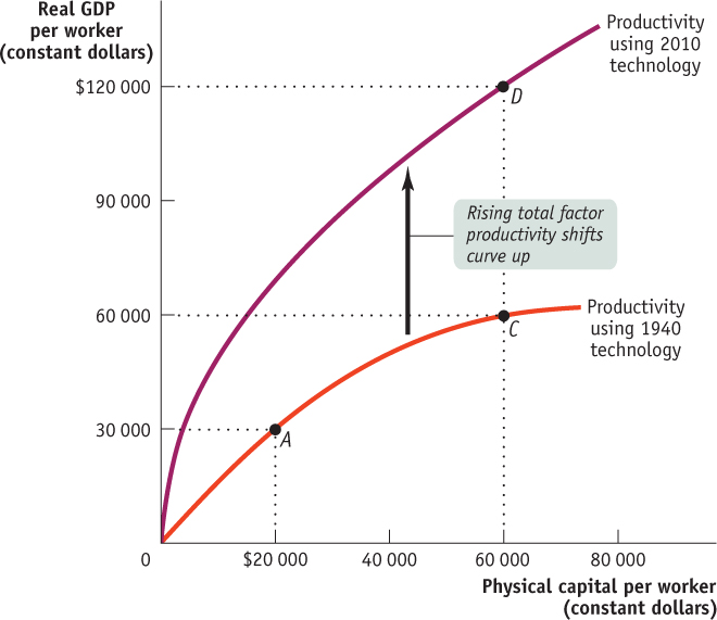
Let’s assume that between 1940 and 2010 the amount of physical capital per worker rose from $20 000 to $60 000. If this increase in physical capital per worker had taken place without any technological progress, the economy would have moved from A to C: output per worker would have risen, but only from $30 000 to $60 000, or 1% per year (using the Rule of 70 tells us that a 1% growth rate over 70 years doubles output). In fact, however, the economy moved from A to D: output rose from $30 000 to $120 000, or 2% per year. There was an increase in both physical capital per worker and technological progress, which shifted the per worker production function.
In this case, 50% of the annual 2% increase in productivity—
Most estimates find that increases in total factor productivity are central to a country’s economic growth in the long-
Figure 9-6 shows the average annual growth in labour productivity for all provinces and territories up to 2011. The average labour productivity growth was 1.2% for Canada as a whole. All regions experienced positive labour productivity growth during this period, but the amount of growth varied significantly. Nunavut enjoyed the highest growth rate, with an annual growth rate of 3.2%. Newfoundland and Labrador had the second highest growth with an annual growth rate of 2.6%. On the other hand, Alberta had the lowest labour productivity growth, at 0.7%. You may find this surprising, given the significant amount of industry in Alberta. So why is that province’s annual growth rate so low?
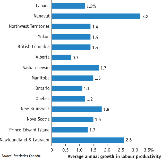
Source: Statistics Canada.
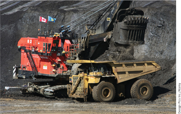
According to Statistics Canada, the answer lies in the rate of accumulation of productive capital or stock of physical capital and total factor productivity growth. During the time frame in question, all regions saw an increase in their physical capital. In fact, Alberta’s (and Saskatchewan’s) physical capital increased by much more than that of the other regions. This is to be expected, because these two provinces are engaged in projects, such as the Alberta oil sands, that are extremely capital-
Some regions grew faster while some grew more slowly. But whether the growth is fast or slow, the bottom line is that higher labour productivity transforms into and reflects higher (per capita) economic growth.
What About Natural Resources?
In our discussion so far, we haven’t mentioned natural resources, which certainly have an effect on productivity. Other things equal, countries that are abundant in valuable natural resources, such as highly fertile land or rich mineral deposits, have higher real GDP per capita than less fortunate countries. The most obvious modern example is the Middle East, where enormous oil deposits have made a few sparsely populated countries very rich. For example, Kuwait has about the same level of real GDP per capita as Germany, but Kuwait’s wealth is based on oil, not manufacturing, the source of Germany’s high real output per worker.
But other things are often not equal. In the modern world, natural resources are a much less important determinant of productivity than human or physical capital for the great majority of countries. For example, some nations with very high real GDP per capita, such as Japan, have very few natural resources. Some resource-rich nations, such as Nigeria (which has sizable oil deposits), are very poor.
Historically, natural resources played a much more prominent role in determining productivity. In the nineteenth century, the countries with the highest real GDP per capita were those abundant in rich farmland and mineral deposits: Canada, the United States, Argentina, and Australia. As a consequence, natural resources figured prominently in the development of economic thought. In a famous book published in 1798, An Essay on the Principle of Population, the English economist Thomas Malthus made the fixed quantity of land in the world the basis of a pessimistic prediction about future productivity. As population grew, he pointed out, the amount of land per worker would decline. And this, other things equal, would cause productivity to fall.
His view, in fact, was that improvements in technology or increases in physical capital would lead only to temporary improvements in productivity because they would always be offset by the pressure of rising population and more workers on the supply of land. In the long run, he concluded, the great majority of people were condemned to living on the edge of starvation. Only then would death rates be high enough and birth rates low enough to prevent rapid population growth from outstripping productivity growth.
It hasn’t turned out that way, although many historians believe that Malthus’s prediction of falling or stagnant productivity was valid for much of human history. Population pressure probably did prevent large productivity increases until the eighteenth century. But in the time since Malthus wrote his book, any negative effects on productivity from population growth have been far outweighed by other, positive factors—advances in technology, increases in human and physical capital, and the opening up of enormous amounts of cultivatable land in the New World.
It remains true, however, that we live on a finite planet, with limited supplies of resources such as oil and limited ability to absorb environmental damage. We address the concerns these limitations pose for economic growth in the final section of this chapter.
THE INFORMATION TECHNOLOGY PARADOX
From the early 1970s through the mid-1990s, Canada went through a slump in growth of both output per worker and total factor productivity. Figure 9-7 shows Statistics Canada estimates of annual labour and total factor productivity growth, averaged for each five-year period from 1962 to 2010. Output per worker is commonly used as a simple proxy for the standard of living of members of a society in the long-run. As Figure 9-7 shows, a significant portion of the growth of output per worker comes from total factor productivity growth. Also, as you can see, there was a large fall in the total factor productivity growth rate beginning in the early 1970s. Because higher total factor productivity plays such a key role in long-run growth, the economy’s overall growth was also disappointing, leading to a widespread sense that economic progress had ground to a halt.
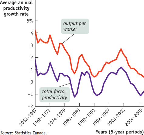
Source: Statistics Canada.
Many economists were puzzled by the slowdown in total factor productivity growth in the early 1970s, since in other ways the era seemed to be one of rapid technological progress. Modern information technology really began with the development of the first microprocessor—a computer on a chip—in 1971. In the 25 years that followed, a series of inventions that seemed revolutionary became standard equipment in the business world: fax machines, desktop computers, cellphones, and e-mail. Yet the rate of growth of total factor productivity remained stagnant. In a famous remark, MIT economics professor and Nobel laureate Robert Solow, a pioneer in the analysis of economic growth, declared that the information technology revolution could be seen everywhere except in the economic statistics.
Why didn’t information technology show large rewards? Paul David, a Stanford University economic historian, offered a theory and a prediction. He pointed out that 100 years earlier another miracle technology—electric power—had spread through the economy, again with surprisingly little impact on productivity growth at first. The reason, he suggested, was that a new technology doesn’t yield its full potential if you use it in old ways.
For example, a traditional factory around 1900 was a multi-storey building, with the machinery tightly crowded together and designed to be powered by a steam engine in the basement. This design had problems: it was very difficult to move people and materials around. Yet owners who electrified their factories initially maintained the multi-storey, tightly packed layout. Only with the switch to spread-out, one-storey factories that took advantage of the flexibility of electric power—most famously Henry Ford’s auto assembly line—did productivity take off.
David suggested that the same phenomenon was happening with information technology. Productivity, he predicted, would take off when people really changed their way of doing business to take advantage of the new technology—such as replacing letters and phone calls with e-mail. Sure enough, productivity growth accelerated dramatically in the second half of the 1990s as companies began to use information technology more effectively.

Quick Review
Long-run increases in living standards arise almost entirely from growing labour productivity, often referred to as the Average Productivity of Labour (APL), or simply productivity.
The positive marginal productivity of physical capital (MPK) is the amount by which productivity is increased as the result of a small increase in physical capital used. An increase in physical capital is one source of higher productivity, but it is subject to diminishing returns to physical capital or diminishing marginal productivity of (physical) capital (dim MPK).
Human capital and technological progress are also sources of increases in productivity.
The per worker production function is used to estimate the sources of increases in productivity. The aggregate production function is a relationship that shows how the aggregate real quantity of output is produced using the available factors of production (the inputs: labour, physical capital, and human capital) and technology [A and the function F(…)]. Growth accounting has shown that rising total factor productivity, interpreted as the effect of technological progress, is central to long-run economic growth.
Natural resources are less import-ant today than physical and human capital as sources of productivity growth in most economies.
Check Your Understanding 9-2
CHECK YOUR UNDERSTANDING 9-2
Predict the effect of each of the following events on the growth rate of productivity.
The amounts of physical and human capital per worker are unchanged, but there is significant technological progress.
The amount of physical capital per worker grows at a steady pace, but the level of human capital per worker and technology are unchanged.
Significant technological progress will result in a positive growth rate of productivity even though physical capital per worker and human capital per worker are unchanged.
The growth rate of productivity will fall but remain positive due to diminishing returns to physical capital.
Output in the economy of Erewhon has grown 3% per year over the past 30 years. The labour force has grown at 1% per year, and the quantity of physical capital has grown at 4% per year. The average education level hasn’t changed. Estimates by economists say that each 1% increase in physical capital per worker, other things equal, raises productivity by 0.3%. (Hint: % change in (X/Y) = % change in X − % change in Y.)
How fast has productivity in Erewhon grown?
How fast has physical capital per worker grown?
How much has growing physical capital per worker contributed to productivity growth? What percentage of productivity growth is that?
How much has technological progress contributed to productivity growth? What percentage of productivity growth is that?
If output has grown 3% per year and the labour force has grown 1% per year, then productivity—output per person—has grown at approximately 3% – 1% = 2% per year.
If physical capital has grown 4% per year and the labour force has grown 1% per year, then physical capital per worker has grown at approximately 4% – 1% = 3% per year.
According to estimates, each 1% rise in physical capital, other things equal, increases productivity by 0.3%. So, as physical capital per worker has increased by 3%, productivity growth that can be attributed to an increase in physical capital per worker is 0.3 × 3% = 0.9%. As a percentage of total productivity growth, this is 0.9%/2% × 100% = 45%.
If the rest of productivity growth is due to technological progress, then technological progress has contributed 2% – 0.9% = 1.1% to productivity growth. As a percentage of total productivity growth, this is 1.1%/2% × 100% = 55%.
Multinomics, Inc., is a large company with many offices around the country. It has just adopted a new computer system that will affect virtually every function performed within the company. Why might a period of time pass before employees’ productivity is improved by the new computer system? Why might there be a temporary decrease in employees’ productivity?
It will take a period time for workers to learn how to use the new computer system and to adjust their routines. And because there are often setbacks in learning a new system, such as accidentally erasing your computer files, productivity at Multinomics may decrease for a period of time.